

178
7 Some Models of “Quantum Measurement”
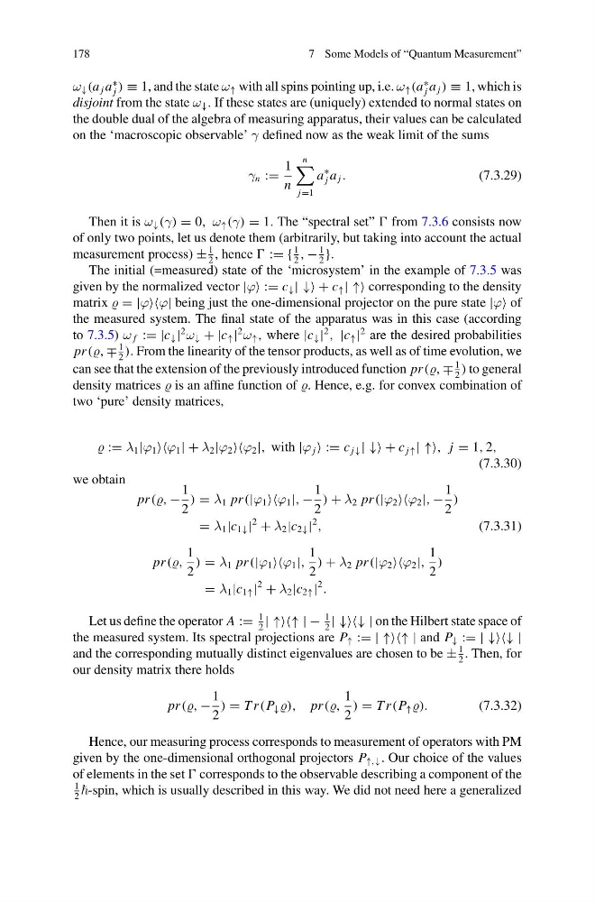
ω ↓ (a j a
∗
j ) ≡ 1, and the state ω ↑ with all spins pointing up, i.e. ω ↑ (a
∗
j a j ) ≡ 1, which is
disjoint from the state ω ↓ . If these states are (uniquely) extended to normal states on
the double dual of the algebra of measuring apparatus, their values can be calculated
on the ‘macroscopic observable’ γ defined now as the weak limit of the sums
γ n :=
1
n
n
j=1
a
∗
j a j .
(7.3.29)
Then it is ω ↓ (γ) = 0, ω ↑ (γ) = 1. The “spectral set” from 7.3.6 consists now
of only two points, let us denote them (arbitrarily, but taking into account the actual
measurement process) ±
1
2
, hence := {
1
2
, −
1
2
}.
The initial (=measured) state of the ‘microsystem’ in the example of 7.3.5 was
given by the normalized vector |ϕ := c ↓ | ↓↓ + c ↑ | ↑↑ corresponding to the density
matrix = |ϕϕ| being just the one-dimensional projector on the pure state |ϕ of
the measured system. The final state of the apparatus was in this case (according
to 7.3.5) ω f := |c ↓ |
2
ω ↓ + |c ↑ |
2
ω ↑ , where |c ↓ |
2
, |c ↑ |
2 are the desired probabilities
pr (, ∓
1
2
). From the linearity of the tensor products, as well as of time evolution, we
can see that the extension of the previously introduced function pr (, ∓
1
2
) to general
density matrices is an affine function of . Hence, e.g. for convex combination of
two ‘pure’ density matrices,
:= λ 1 |ϕ 1 ϕ 1 | + λ 2 |ϕ 2 ϕ 2 |, with |ϕ j := c j↓ | ↓↓ + c j↑ | ↑↑, j = 1, 2,
(7.3.30)
we obtain
pr (, −
1
2
) = λ 1 pr (|ϕ 1 ϕ 1 |, −
1
2
) + λ 2 pr (|ϕ 2 ϕ 2 |, −
1
2
)
= λ 1 |c 1↓ |
2
+ λ 2 |c 2↓ |
2
,
(7.3.31)
pr (,
1
2
) = λ 1 pr (|ϕ 1 ϕ 1 |,
1
2
) + λ 2 pr (|ϕ 2 ϕ 2 |,
1
2
)
= λ 1 |c 1↑ |
2
+ λ 2 |c 2↑ |
2
.
Let us define the operator A :=
1
2
| ↑↑↑↑ | −
1
2
| ↓↓↓↓ | on the Hilbert state space of
the measured system. Its spectral projections are P ↑ := | ↑↑↑↑ | and P ↓ := | ↓↓↓↓ |
and the corresponding mutually distinct eigenvalues are chosen to be ±
1
2
. Then, for
our density matrix there holds
pr (, −
1
2
) = T r(P ↓ ), pr (,
1
2
) = T r(P ↑ ).
(7.3.32)
Hence, our measuring process corresponds to measurement of operators with PM
given by the one-dimensional orthogonal projectors P ↑,↓ . Our choice of the values
of elements in the set corresponds to the observable describing a component of the
1
2
-spin, which is usually described in this way. We did not need here a generalized
7 Some Models of “Quantum Measurement”
ω ↓ (a j a
∗
j ) ≡ 1, and the state ω ↑ with all spins pointing up, i.e. ω ↑ (a
∗
j a j ) ≡ 1, which is
disjoint from the state ω ↓ . If these states are (uniquely) extended to normal states on
the double dual of the algebra of measuring apparatus, their values can be calculated
on the ‘macroscopic observable’ γ defined now as the weak limit of the sums
γ n :=
1
n
n
j=1
a
∗
j a j .
(7.3.29)
Then it is ω ↓ (γ) = 0, ω ↑ (γ) = 1. The “spectral set” from 7.3.6 consists now
of only two points, let us denote them (arbitrarily, but taking into account the actual
measurement process) ±
1
2
, hence := {
1
2
, −
1
2
}.
The initial (=measured) state of the ‘microsystem’ in the example of 7.3.5 was
given by the normalized vector |ϕ := c ↓ | ↓↓ + c ↑ | ↑↑ corresponding to the density
matrix = |ϕϕ| being just the one-dimensional projector on the pure state |ϕ of
the measured system. The final state of the apparatus was in this case (according
to 7.3.5) ω f := |c ↓ |
2
ω ↓ + |c ↑ |
2
ω ↑ , where |c ↓ |
2
, |c ↑ |
2 are the desired probabilities
pr (, ∓
1
2
). From the linearity of the tensor products, as well as of time evolution, we
can see that the extension of the previously introduced function pr (, ∓
1
2
) to general
density matrices is an affine function of . Hence, e.g. for convex combination of
two ‘pure’ density matrices,
:= λ 1 |ϕ 1 ϕ 1 | + λ 2 |ϕ 2 ϕ 2 |, with |ϕ j := c j↓ | ↓↓ + c j↑ | ↑↑, j = 1, 2,
(7.3.30)
we obtain
pr (, −
1
2
) = λ 1 pr (|ϕ 1 ϕ 1 |, −
1
2
) + λ 2 pr (|ϕ 2 ϕ 2 |, −
1
2
)
= λ 1 |c 1↓ |
2
+ λ 2 |c 2↓ |
2
,
(7.3.31)
pr (,
1
2
) = λ 1 pr (|ϕ 1 ϕ 1 |,
1
2
) + λ 2 pr (|ϕ 2 ϕ 2 |,
1
2
)
= λ 1 |c 1↑ |
2
+ λ 2 |c 2↑ |
2
.
Let us define the operator A :=
1
2
| ↑↑↑↑ | −
1
2
| ↓↓↓↓ | on the Hilbert state space of
the measured system. Its spectral projections are P ↑ := | ↑↑↑↑ | and P ↓ := | ↓↓↓↓ |
and the corresponding mutually distinct eigenvalues are chosen to be ±
1
2
. Then, for
our density matrix there holds
pr (, −
1
2
) = T r(P ↓ ), pr (,
1
2
) = T r(P ↑ ).
(7.3.32)
Hence, our measuring process corresponds to measurement of operators with PM
given by the one-dimensional orthogonal projectors P ↑,↓ . Our choice of the values
of elements in the set corresponds to the observable describing a component of the
1
2
-spin, which is usually described in this way. We did not need here a generalized