

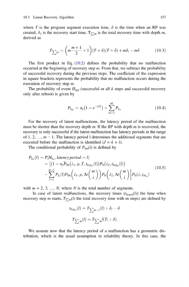
where T is the program segment execution time, d is the time when an RP was
created, d 1 is the recovery start time, T
P
m is the total recovery time with depth m,
derived as
T P
m ¼ m
m þ 1
2
þ 1
T þ d
ð
Þ T þ d
ð
Þþmd i À md
ð10:3Þ
The first product in Eq. (10.2) defines the probability that no malfunction
occurred at the beginning of recovery step m. From that, we subtract the probability
of successful recovery during the previous steps. The coefficient of the expression
in square brackets represents the probability that no malfunction occurs during the
execution of recovery step m.
The probability of event H kpf (successful or all k steps and successful recovery
only after reboot) is given by
P k pf ¼ a k 1 À e
ÀikT
À
Á
À
X nk
m¼1
P k m
ð10:4Þ
For the recovery of latent malfunctions, the latency period of the malfunction
must be shorter than the recovery depth m. If the RP with depth m is recovered, the
recovery is only successful if the latent malfunction has latency periods in the range
of 1, 2, …, m − 1. The latency period l determines the additional segments that are
executed before the malfunction is identified (J = k + l).
The conditional probability of P km (l) is defined by
P k m ðlÞ ¼ P H k m ; latency period ¼ l
½
Þ
¼ ð1 À a k P 00 k 1 ; l; T; t beg m ðlÞ
À
Á
P 0 k 2 ; t beg m ðlÞ
À
Á
Â
À
X mÀ1
i¼1
P k i ðlÞP 00 k 1 ; l; Dt
m
i
P 0 k 2 ; Dt
m
i
!
P 0 k; t rb m
ð
Þ
ð10:5Þ
with m = 2, 3, …, N, where N is the total number of segments.
In case of latent malfunctions, the recovery times (t begm (l)) the time when
recovery step m starts, T P
m (l) the total recovery time with m steps) are defined by
t beg m ðlÞ ¼ T P
mÀ1 ðlÞ þ d i À d
T P
m ðlÞ ¼ T P
m l T i þ d
ð
Þ
We assume now that the latency period of a malfunction has a geometric distribution, which is the usual assumption in reliability theory. In this case, the
10.3 Linear Recovery Algorithm
157
created, d 1 is the recovery start time, T
P
m is the total recovery time with depth m,
derived as
T P
m ¼ m
m þ 1
2
þ 1
T þ d
ð
Þ T þ d
ð
Þþmd i À md
ð10:3Þ
The first product in Eq. (10.2) defines the probability that no malfunction
occurred at the beginning of recovery step m. From that, we subtract the probability
of successful recovery during the previous steps. The coefficient of the expression
in square brackets represents the probability that no malfunction occurs during the
execution of recovery step m.
The probability of event H kpf (successful or all k steps and successful recovery
only after reboot) is given by
P k pf ¼ a k 1 À e
ÀikT
À
Á
À
X nk
m¼1
P k m
ð10:4Þ
For the recovery of latent malfunctions, the latency period of the malfunction
must be shorter than the recovery depth m. If the RP with depth m is recovered, the
recovery is only successful if the latent malfunction has latency periods in the range
of 1, 2, …, m − 1. The latency period l determines the additional segments that are
executed before the malfunction is identified (J = k + l).
The conditional probability of P km (l) is defined by
P k m ðlÞ ¼ P H k m ; latency period ¼ l
½
Þ
¼ ð1 À a k P 00 k 1 ; l; T; t beg m ðlÞ
À
Á
P 0 k 2 ; t beg m ðlÞ
À
Á
Â
À
X mÀ1
i¼1
P k i ðlÞP 00 k 1 ; l; Dt
m
i
P 0 k 2 ; Dt
m
i
!
P 0 k; t rb m
ð
Þ
ð10:5Þ
with m = 2, 3, …, N, where N is the total number of segments.
In case of latent malfunctions, the recovery times (t begm (l)) the time when
recovery step m starts, T P
m (l) the total recovery time with m steps) are defined by
t beg m ðlÞ ¼ T P
mÀ1 ðlÞ þ d i À d
T P
m ðlÞ ¼ T P
m l T i þ d
ð
Þ
We assume now that the latency period of a malfunction has a geometric distribution, which is the usual assumption in reliability theory. In this case, the
10.3 Linear Recovery Algorithm
157