

10.3 Linear Recovery Algorithm
The linear recovery method is based on linear search and is described in detail in
[2–7]. We give here just a short summary of the algorithm. If the checking logic
detects a malfunction at the end of segment J, the computation is interrupted,
RP (j − 1) is recovered and the processing resumed.
If during the repeated execution the checking logic does not detect the malfunction again, the recovery is assumed to be successful and the system continues
by executing segment (J + 1).
If the malfunction is detected again, the interrupted process is resumed from RP
(J − 2), etc., until a correct RP is reached which has been established without
including information corrupted by the malfunction.
The difference to the MLR lies in the way recovery is performed. MLR uses the
checksums to identify changes in the execution, whereas the linear approach always
re-executes all code fragments until the end of execution when the checking logic
signaled the fault.
The probability that one of the events H c , H m , H m (L), H pf , or H pf (L) occurs is
estimated with the aid of Sect. 3.1 and adopted from [7, 8].
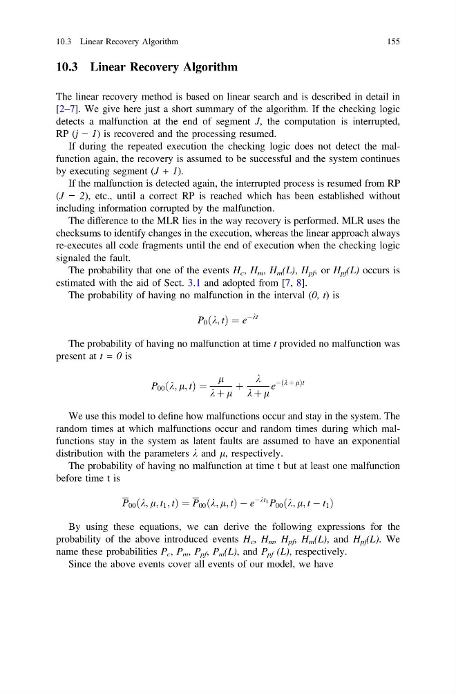
The probability of having no malfunction in the interval (0, t) is
P 0 ðk; tÞ ¼ e
Àkt
The probability of having no malfunction at time t provided no malfunction was
present at t = 0 is
P 00 k; l; t
ð
Þ¼
l
k þ l
þ
k
k þ l
e
À k þ l
ð
Þ t
We use this model to define how malfunctions occur and stay in the system. The
random times at which malfunctions occur and random times during which malfunctions stay in the system as latent faults are assumed to have an exponential
distribution with the parameters k and l, respectively.
The probability of having no malfunction at time t but at least one malfunction
before time t is
P 00 k; l; t 1 ; t
ð
Þ¼P 00 k; l; t
ð
ÞÀe
Àkt 1 P 00 k; l; t À t 1
ð
Þ
By using these equations, we can derive the following expressions for the
probability of the above introduced events H c , H m , H pf , H m (L), and H pf (L). We
name these probabilities P c , P m , P pf , P m (L), and P pf (L), respectively.
Since the above events cover all events of our model, we have
10.3 Linear Recovery Algorithm
155
The linear recovery method is based on linear search and is described in detail in
[2–7]. We give here just a short summary of the algorithm. If the checking logic
detects a malfunction at the end of segment J, the computation is interrupted,
RP (j − 1) is recovered and the processing resumed.
If during the repeated execution the checking logic does not detect the malfunction again, the recovery is assumed to be successful and the system continues
by executing segment (J + 1).
If the malfunction is detected again, the interrupted process is resumed from RP
(J − 2), etc., until a correct RP is reached which has been established without
including information corrupted by the malfunction.
The difference to the MLR lies in the way recovery is performed. MLR uses the
checksums to identify changes in the execution, whereas the linear approach always
re-executes all code fragments until the end of execution when the checking logic
signaled the fault.
The probability that one of the events H c , H m , H m (L), H pf , or H pf (L) occurs is
estimated with the aid of Sect. 3.1 and adopted from [7, 8].
The probability of having no malfunction in the interval (0, t) is
P 0 ðk; tÞ ¼ e
Àkt
The probability of having no malfunction at time t provided no malfunction was
present at t = 0 is
P 00 k; l; t
ð
Þ¼
l
k þ l
þ
k
k þ l
e
À k þ l
ð
Þ t
We use this model to define how malfunctions occur and stay in the system. The
random times at which malfunctions occur and random times during which malfunctions stay in the system as latent faults are assumed to have an exponential
distribution with the parameters k and l, respectively.
The probability of having no malfunction at time t but at least one malfunction
before time t is
P 00 k; l; t 1 ; t
ð
Þ¼P 00 k; l; t
ð
ÞÀe
Àkt 1 P 00 k; l; t À t 1
ð
Þ
By using these equations, we can derive the following expressions for the
probability of the above introduced events H c , H m , H pf , H m (L), and H pf (L). We
name these probabilities P c , P m , P pf , P m (L), and P pf (L), respectively.
Since the above events cover all events of our model, we have
10.3 Linear Recovery Algorithm
155