

index ¼
Dk max À Dk est
ð
Þ k c
n
ð8:2Þ
The constraints of this formula must of course also be taken into account. For
example, if the current malfunction rate Δk c is below Δk est , the lowest reliability
mode be chosen.
The formula above can be easily replaced by other functions, as needed.
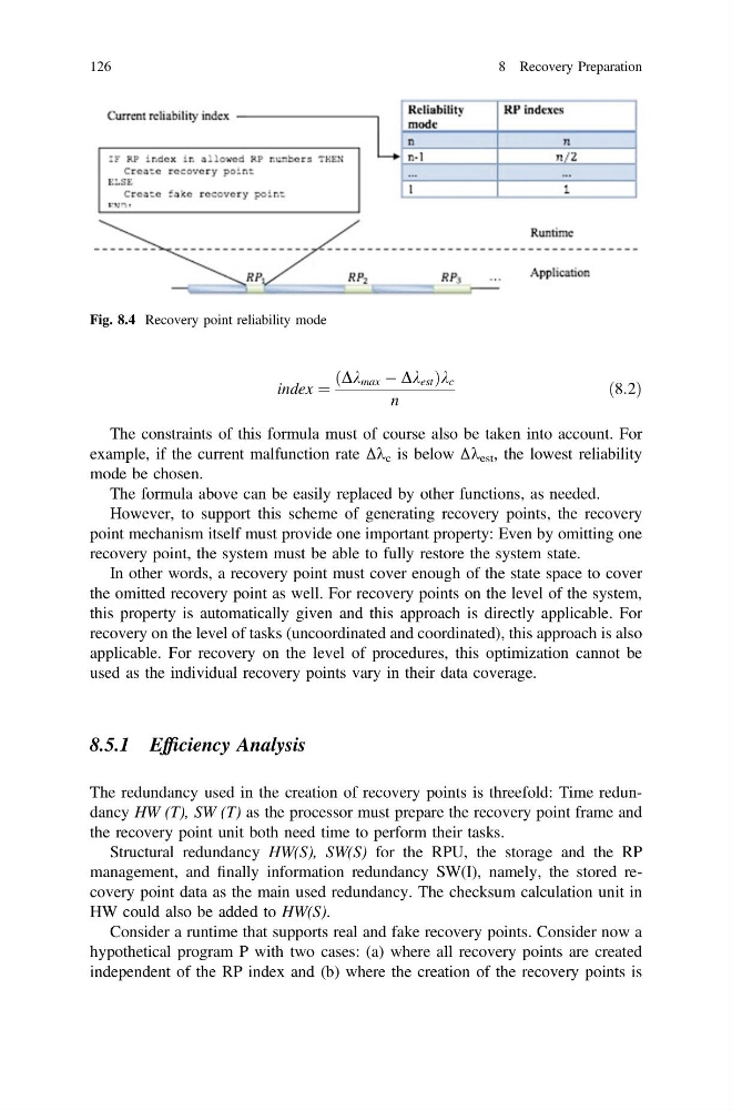
However, to support this scheme of generating recovery points, the recovery
point mechanism itself must provide one important property: Even by omitting one
recovery point, the system must be able to fully restore the system state.
In other words, a recovery point must cover enough of the state space to cover
the omitted recovery point as well. For recovery points on the level of the system,
this property is automatically given and this approach is directly applicable. For
recovery on the level of tasks (uncoordinated and coordinated), this approach is also
applicable. For recovery on the level of procedures, this optimization cannot be
used as the individual recovery points vary in their data coverage.
8.5.1 Efficiency Analysis
The redundancy used in the creation of recovery points is threefold: Time redundancy HW (T), SW (T) as the processor must prepare the recovery point frame and
the recovery point unit both need time to perform their tasks.
Structural redundancy HW(S), SW(S) for the RPU, the storage and the RP
management, and finally information redundancy SW(I), namely, the stored recovery point data as the main used redundancy. The checksum calculation unit in
HW could also be added to HW(S).
Consider a runtime that supports real and fake recovery points. Consider now a
hypothetical program P with two cases: (a) where all recovery points are created
independent of the RP index and (b) where the creation of the recovery points is
Fig. 8.4 Recovery point reliability mode
126
8 Recovery Preparation
Dk max À Dk est
ð
Þ k c
n
ð8:2Þ
The constraints of this formula must of course also be taken into account. For
example, if the current malfunction rate Δk c is below Δk est , the lowest reliability
mode be chosen.
The formula above can be easily replaced by other functions, as needed.
However, to support this scheme of generating recovery points, the recovery
point mechanism itself must provide one important property: Even by omitting one
recovery point, the system must be able to fully restore the system state.
In other words, a recovery point must cover enough of the state space to cover
the omitted recovery point as well. For recovery points on the level of the system,
this property is automatically given and this approach is directly applicable. For
recovery on the level of tasks (uncoordinated and coordinated), this approach is also
applicable. For recovery on the level of procedures, this optimization cannot be
used as the individual recovery points vary in their data coverage.
8.5.1 Efficiency Analysis
The redundancy used in the creation of recovery points is threefold: Time redundancy HW (T), SW (T) as the processor must prepare the recovery point frame and
the recovery point unit both need time to perform their tasks.
Structural redundancy HW(S), SW(S) for the RPU, the storage and the RP
management, and finally information redundancy SW(I), namely, the stored recovery point data as the main used redundancy. The checksum calculation unit in
HW could also be added to HW(S).
Consider a runtime that supports real and fake recovery points. Consider now a
hypothetical program P with two cases: (a) where all recovery points are created
independent of the RP index and (b) where the creation of the recovery points is
Fig. 8.4 Recovery point reliability mode
126
8 Recovery Preparation