

4.3 Coordinate Transformation in Plates and Shells
63
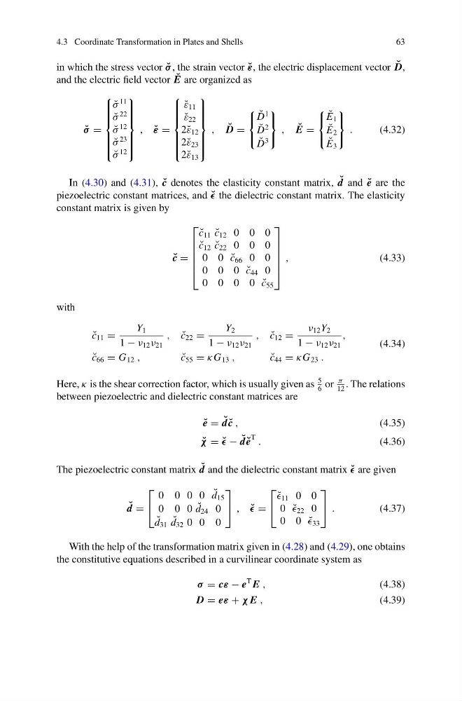
in which the stress vector ˘
σ , the strain vector ˘
ε, the electric displacement vector ˘
D,
and the electric field vector ˘
E are organized as
˘
σ =
⎧
⎪ ⎪ ⎪ ⎪ ⎨
⎪ ⎪ ⎪ ⎪ ⎩
˘
σ
11
˘
σ
22
˘
σ
12
˘
σ
23
˘
σ
12
⎫
⎪ ⎪ ⎪ ⎪ ⎬
⎪ ⎪ ⎪ ⎪ ⎭
, ˘
ε =
⎧
⎪ ⎪ ⎪ ⎪ ⎨
⎪ ⎪ ⎪ ⎪ ⎩
˘
ε 11
˘
ε 22
2˘ ε 12
2˘ ε 23
2˘ ε 13
⎫
⎪ ⎪ ⎪ ⎪ ⎬
⎪ ⎪ ⎪ ⎪ ⎭
, ˘
D =
⎧
⎨
⎩
˘
D
1
˘
D
2
˘
D
3
⎫
⎬
⎭
, ˘
E =
⎧
⎨
⎩
˘
E 1
˘
E 2
˘
E 3
⎫
⎬
⎭
.
(4.32)
In (4.30) and (4.31), ˘
c denotes the elasticity constant matrix, ˘
d and ˘
e are the
piezoelectric constant matrices, and ˘
the dielectric constant matrix. The elasticity
constant matrix is given by
˘
c =
⎡
⎢
⎢
⎢
⎢
⎣
˘
c 11 ˘
c 12 0 0 0
˘
c 12 ˘
c 22 0 0 0
0 0 ˘
c 66 0 0
0 0 0 ˘
c 44 0
0 0 0 0 ˘
c 55
⎤
⎥
⎥
⎥
⎥
⎦
,
(4.33)
with
˘
c 11 =
Y 1
1 − ν 12 ν 21
, ˘
c 22 =
Y 2
1 − ν 12 ν 21
, ˘
c 12 =
ν 12 Y 2
1 − ν 12 ν 21
,
˘
c 66 = G 12 ,
˘
c 55 = κG 13 ,
˘
c 44 = κG 23 .
(4.34)
Here, κ is the shear correction factor, which is usually given as
5
6
or
π
12
. The relations
between piezoelectric and dielectric constant matrices are
˘
e = ˘
d ˘
c ,
(4.35)
˘
χ = ˘
− ˘
d ˘
e
T .
(4.36)
The piezoelectric constant matrix ˘
d and the dielectric constant matrix ˘
are given
˘
d =
⎡
⎣
0 0 0 0 ˘
d 15
0 0 0 ˘
d 24 0
˘
d 31 ˘
d 32 0 0 0
⎤
⎦ , ˘
=
⎡
⎣
˘
11 0 0
0 ˘
22 0
0 0 ˘
33
⎤
⎦ .
(4.37)
With the help of the transformation matrix given in (4.28) and (4.29), one obtains
the constitutive equations described in a curvilinear coordinate system as
σ = cε − e
T E ,
(4.38)
D = eε + χ E ,
(4.39)
63
in which the stress vector ˘
σ , the strain vector ˘
ε, the electric displacement vector ˘
D,
and the electric field vector ˘
E are organized as
˘
σ =
⎧
⎪ ⎪ ⎪ ⎪ ⎨
⎪ ⎪ ⎪ ⎪ ⎩
˘
σ
11
˘
σ
22
˘
σ
12
˘
σ
23
˘
σ
12
⎫
⎪ ⎪ ⎪ ⎪ ⎬
⎪ ⎪ ⎪ ⎪ ⎭
, ˘
ε =
⎧
⎪ ⎪ ⎪ ⎪ ⎨
⎪ ⎪ ⎪ ⎪ ⎩
˘
ε 11
˘
ε 22
2˘ ε 12
2˘ ε 23
2˘ ε 13
⎫
⎪ ⎪ ⎪ ⎪ ⎬
⎪ ⎪ ⎪ ⎪ ⎭
, ˘
D =
⎧
⎨
⎩
˘
D
1
˘
D
2
˘
D
3
⎫
⎬
⎭
, ˘
E =
⎧
⎨
⎩
˘
E 1
˘
E 2
˘
E 3
⎫
⎬
⎭
.
(4.32)
In (4.30) and (4.31), ˘
c denotes the elasticity constant matrix, ˘
d and ˘
e are the
piezoelectric constant matrices, and ˘
the dielectric constant matrix. The elasticity
constant matrix is given by
˘
c =
⎡
⎢
⎢
⎢
⎢
⎣
˘
c 11 ˘
c 12 0 0 0
˘
c 12 ˘
c 22 0 0 0
0 0 ˘
c 66 0 0
0 0 0 ˘
c 44 0
0 0 0 0 ˘
c 55
⎤
⎥
⎥
⎥
⎥
⎦
,
(4.33)
with
˘
c 11 =
Y 1
1 − ν 12 ν 21
, ˘
c 22 =
Y 2
1 − ν 12 ν 21
, ˘
c 12 =
ν 12 Y 2
1 − ν 12 ν 21
,
˘
c 66 = G 12 ,
˘
c 55 = κG 13 ,
˘
c 44 = κG 23 .
(4.34)
Here, κ is the shear correction factor, which is usually given as
5
6
or
π
12
. The relations
between piezoelectric and dielectric constant matrices are
˘
e = ˘
d ˘
c ,
(4.35)
˘
χ = ˘
− ˘
d ˘
e
T .
(4.36)
The piezoelectric constant matrix ˘
d and the dielectric constant matrix ˘
are given
˘
d =
⎡
⎣
0 0 0 0 ˘
d 15
0 0 0 ˘
d 24 0
˘
d 31 ˘
d 32 0 0 0
⎤
⎦ , ˘
=
⎡
⎣
˘
11 0 0
0 ˘
22 0
0 0 ˘
33
⎤
⎦ .
(4.37)
With the help of the transformation matrix given in (4.28) and (4.29), one obtains
the constitutive equations described in a curvilinear coordinate system as
σ = cε − e
T E ,
(4.38)
D = eε + χ E ,
(4.39)