

2 Peridynamic Simulation for Thermal and Mechanical Behavior …
19
2.2 Description of Physical Mechanism
The physical phenomena in MIG welding process of a manufactured structure,
contains essentially the thermal transfer and mechanical distortion problems. Those
related physical mechanisms are usually supposed to solve on the basis of a weak
coupled thermo-mechanical modeling, in which the change of temperature field will
generate the linear expansion of materials, however, the material deformation does
not influence temperature field in converse. In addition, the geometrical discontinuities and boundaries are changed in the wake of welding process. To overcome the
problems mentioned above, the peridynamic method is applied to simulate the MIG
welding process due to its capacity of solving thermo-mechanical problems and
advantage of dealing with geometrical discontinuities. The corresponding expressions of the thermo-mechanical problems in peridynamics are expounded in the
following.
2.2.1 Heat Transfer Mechanism
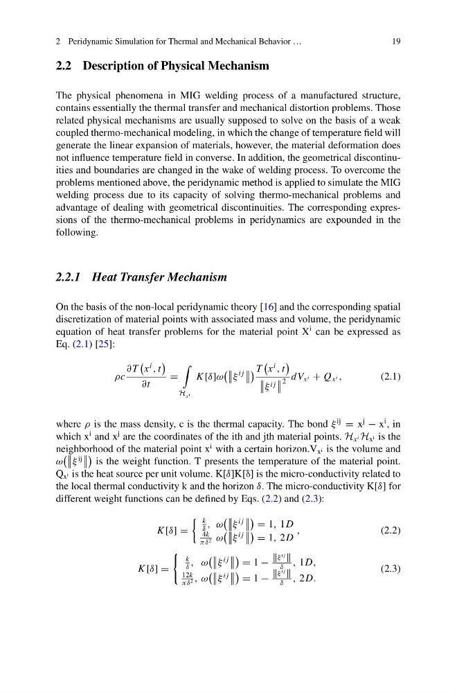
On the basis of the non-local peridynamic theory [16] and the corresponding spatial
discretization of material points with associated mass and volume, the peridynamic
equation of heat transfer problems for the material point X
i can be expressed as
Eq. (2.1) [25]:
ρc
∂ T
x
i
, t
∂t
=
H x i
K [δ]ω
ξ
i j
T
x
i
, t
ξ i j
2 dV x i + Q x i ,
(2.1)
where ρ is the mass density, c is the thermal capacity. The bond ξ
ij
= x
j
− x
i , in
which x
i and x
j are the coordinates of the ith and jth material points. H x i H x i is the
neighborhood of the material point x
i with a certain horizon.V x i is the volume and
ω
ξ
ij
is the weight function. T presents the temperature of the material point.
Q x i is the heat source per unit volume. K[δ]K[δ] is the micro-conductivity related to
the local thermal conductivity k and the horizon δ. The micro-conductivity K[δ] for
different weight functions can be defined by Eqs. (2.2) and (2.3):
K [δ] =
k
δ
, ω
ξ
i j
= 1, 1D
4k
πδ 2 ω
ξ
i j
= 1, 2D
,
(2.2)
K [δ] =
k
δ
, ω
ξ
i j
= 1 −
ξ
i j
δ
, 1D,
12k
πδ 2 , ω
ξ
i j
= 1 −
ξ
i j
δ
, 2D.
(2.3)
19
2.2 Description of Physical Mechanism
The physical phenomena in MIG welding process of a manufactured structure,
contains essentially the thermal transfer and mechanical distortion problems. Those
related physical mechanisms are usually supposed to solve on the basis of a weak
coupled thermo-mechanical modeling, in which the change of temperature field will
generate the linear expansion of materials, however, the material deformation does
not influence temperature field in converse. In addition, the geometrical discontinuities and boundaries are changed in the wake of welding process. To overcome the
problems mentioned above, the peridynamic method is applied to simulate the MIG
welding process due to its capacity of solving thermo-mechanical problems and
advantage of dealing with geometrical discontinuities. The corresponding expressions of the thermo-mechanical problems in peridynamics are expounded in the
following.
2.2.1 Heat Transfer Mechanism
On the basis of the non-local peridynamic theory [16] and the corresponding spatial
discretization of material points with associated mass and volume, the peridynamic
equation of heat transfer problems for the material point X
i can be expressed as
Eq. (2.1) [25]:
ρc
∂ T
x
i
, t
∂t
=
H x i
K [δ]ω
ξ
i j
T
x
i
, t
ξ i j
2 dV x i + Q x i ,
(2.1)
where ρ is the mass density, c is the thermal capacity. The bond ξ
ij
= x
j
− x
i , in
which x
i and x
j are the coordinates of the ith and jth material points. H x i H x i is the
neighborhood of the material point x
i with a certain horizon.V x i is the volume and
ω
ξ
ij
is the weight function. T presents the temperature of the material point.
Q x i is the heat source per unit volume. K[δ]K[δ] is the micro-conductivity related to
the local thermal conductivity k and the horizon δ. The micro-conductivity K[δ] for
different weight functions can be defined by Eqs. (2.2) and (2.3):
K [δ] =
k
δ
, ω
ξ
i j
= 1, 1D
4k
πδ 2 ω
ξ
i j
= 1, 2D
,
(2.2)
K [δ] =
k
δ
, ω
ξ
i j
= 1 −
ξ
i j
δ
, 1D,
12k
πδ 2 , ω
ξ
i j
= 1 −
ξ
i j
δ
, 2D.
(2.3)