

20 Multi-Objective Optimization of Automotive Front Rail …
255
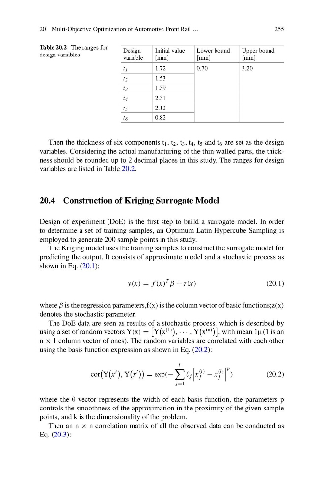
Table 20.2 The ranges for
design variables
Design
variable
Initial value
[mm]
Lower bound
[mm]
Upper bound
[mm]
t 1
1.72
0.70
3.20
t 2
1.53
t 3
1.39
t 4
2.31
t 5
2.12
t 6
0.82
Then the thickness of six components t 1 , t 2 , t 3 , t 4 , t 5 and t 6 are set as the design
variables. Considering the actual manufacturing of the thin-walled parts, the thickness should be rounded up to 2 decimal places in this study. The ranges for design
variables are listed in Table 20.2.
20.4 Construction of Kriging Surrogate Model
Design of experiment (DoE) is the first step to build a surrogate model. In order
to determine a set of training samples, an Optimum Latin Hypercube Sampling is
employed to generate 200 sample points in this study.
The Kriging model uses the training samples to construct the surrogate model for
predicting the output. It consists of approximate model and a stochastic process as
shown in Eq. (20.1):
y(x) = f (x)
T
β + z(x)
(20.1)
where β is the regression parameters,f(x) is the column vector of basic functions;z(x)
denotes the stochastic parameter.
The DoE data are seen as results of a stochastic process, which is described by
using a set of random vectors Y(x) =
Y
x
(1)
, · · · , Y
x
(n)
, with mean 1μ(1 is an
n × 1 column vector of ones). The random variables are correlated with each other
using the basis function expression as shown in Eq. (20.2):
cor
Y
x
i
, Y
x
l
= exp(−
k
j=1
θ j
x
(i)
j − x
(l)
j
p )
(20.2)
where the θ vector represents the width of each basis function, the parameters p
controls the smoothness of the approximation in the proximity of the given sample
points, and k is the dimensionality of the problem.
Then an n × n correlation matrix of all the observed data can be conducted as
Eq. (20.3):
255
Table 20.2 The ranges for
design variables
Design
variable
Initial value
[mm]
Lower bound
[mm]
Upper bound
[mm]
t 1
1.72
0.70
3.20
t 2
1.53
t 3
1.39
t 4
2.31
t 5
2.12
t 6
0.82
Then the thickness of six components t 1 , t 2 , t 3 , t 4 , t 5 and t 6 are set as the design
variables. Considering the actual manufacturing of the thin-walled parts, the thickness should be rounded up to 2 decimal places in this study. The ranges for design
variables are listed in Table 20.2.
20.4 Construction of Kriging Surrogate Model
Design of experiment (DoE) is the first step to build a surrogate model. In order
to determine a set of training samples, an Optimum Latin Hypercube Sampling is
employed to generate 200 sample points in this study.
The Kriging model uses the training samples to construct the surrogate model for
predicting the output. It consists of approximate model and a stochastic process as
shown in Eq. (20.1):
y(x) = f (x)
T
β + z(x)
(20.1)
where β is the regression parameters,f(x) is the column vector of basic functions;z(x)
denotes the stochastic parameter.
The DoE data are seen as results of a stochastic process, which is described by
using a set of random vectors Y(x) =
Y
x
(1)
, · · · , Y
x
(n)
, with mean 1μ(1 is an
n × 1 column vector of ones). The random variables are correlated with each other
using the basis function expression as shown in Eq. (20.2):
cor
Y
x
i
, Y
x
l
= exp(−
k
j=1
θ j
x
(i)
j − x
(l)
j
p )
(20.2)
where the θ vector represents the width of each basis function, the parameters p
controls the smoothness of the approximation in the proximity of the given sample
points, and k is the dimensionality of the problem.
Then an n × n correlation matrix of all the observed data can be conducted as
Eq. (20.3):