

44
2 Description of the Wolfram SystemModeler
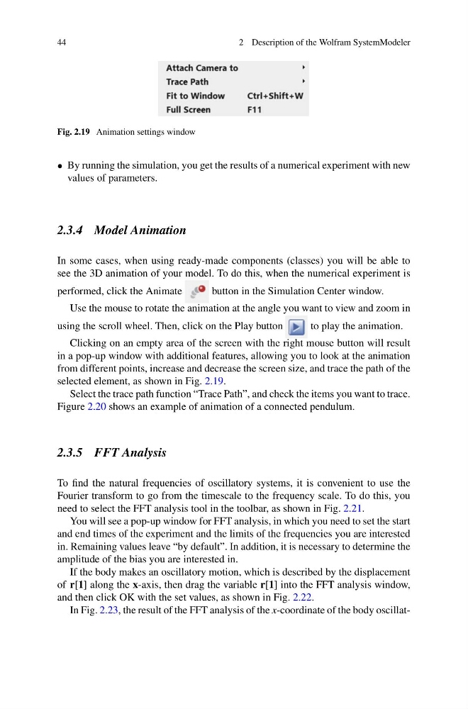
Fig. 2.19 Animation settings window
• By running the simulation, you get the results of a numerical experiment with new
values of parameters.
2.3.4 Model Animation
In some cases, when using ready-made components (classes) you will be able to
see the 3D animation of your model. To do this, when the numerical experiment is
performed, click the Animate
button in the Simulation Center window.
Use the mouse to rotate the animation at the angle you want to view and zoom in
using the scroll wheel. Then, click on the Play button
to play the animation.
Clicking on an empty area of the screen with the right mouse button will result
in a pop-up window with additional features, allowing you to look at the animation
from different points, increase and decrease the screen size, and trace the path of the
selected element, as shown in Fig. 2.19.
Select the trace path function “Trace Path”, and check the items you want to trace.
Figure 2.20 shows an example of animation of a connected pendulum.
2.3.5 FFT Analysis
To find the natural frequencies of oscillatory systems, it is convenient to use the
Fourier transform to go from the timescale to the frequency scale. To do this, you
need to select the FFT analysis tool in the toolbar, as shown in Fig. 2.21.
You will see a pop-up window for FFT analysis, in which you need to set the start
and end times of the experiment and the limits of the frequencies you are interested
in. Remaining values leave “by default”. In addition, it is necessary to determine the
amplitude of the bias you are interested in.
If the body makes an oscillatory motion, which is described by the displacement
of r[1] along the x-axis, then drag the variable r[1] into the FFT analysis window,
and then click OK with the set values, as shown in Fig. 2.22.
In Fig. 2.23, the result of the FFT analysis of the x-coordinate of the body oscillat-
2 Description of the Wolfram SystemModeler
Fig. 2.19 Animation settings window
• By running the simulation, you get the results of a numerical experiment with new
values of parameters.
2.3.4 Model Animation
In some cases, when using ready-made components (classes) you will be able to
see the 3D animation of your model. To do this, when the numerical experiment is
performed, click the Animate
button in the Simulation Center window.
Use the mouse to rotate the animation at the angle you want to view and zoom in
using the scroll wheel. Then, click on the Play button
to play the animation.
Clicking on an empty area of the screen with the right mouse button will result
in a pop-up window with additional features, allowing you to look at the animation
from different points, increase and decrease the screen size, and trace the path of the
selected element, as shown in Fig. 2.19.
Select the trace path function “Trace Path”, and check the items you want to trace.
Figure 2.20 shows an example of animation of a connected pendulum.
2.3.5 FFT Analysis
To find the natural frequencies of oscillatory systems, it is convenient to use the
Fourier transform to go from the timescale to the frequency scale. To do this, you
need to select the FFT analysis tool in the toolbar, as shown in Fig. 2.21.
You will see a pop-up window for FFT analysis, in which you need to set the start
and end times of the experiment and the limits of the frequencies you are interested
in. Remaining values leave “by default”. In addition, it is necessary to determine the
amplitude of the bias you are interested in.
If the body makes an oscillatory motion, which is described by the displacement
of r[1] along the x-axis, then drag the variable r[1] into the FFT analysis window,
and then click OK with the set values, as shown in Fig. 2.22.
In Fig. 2.23, the result of the FFT analysis of the x-coordinate of the body oscillat-