

5.4 Connected Pendulums
173
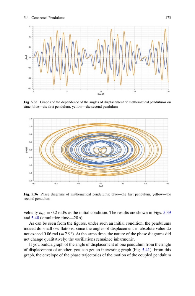
Fig. 5.35 Graphs of the dependence of the angles of displacement of mathematical pendulums on
time: blue—the first pendulum, yellow—the second pendulum
Fig. 5.36 Phase diagrams of mathematical pendulums: blue—the first pendulum, yellow—the
second pendulum
velocity ω x0 = 0.2 rad/s as the initial condition. The results are shown in Figs. 5.39
and 5.40 (simulation time—20 s).
As can be seen from the figures, under such an initial condition, the pendulums
indeed do small oscillations, since the angles of displacement in absolute value do
not exceed 0.06 rad (= 2.9°). At the same time, the nature of the phase diagrams did
not change qualitatively; the oscillations remained inharmonic.
If you build a graph of the angle of displacement of one pendulum from the angle
of displacement of another, you can get an interesting graph (Fig. 5.41). From this
graph, the envelope of the phase trajectories of the motion of the coupled pendulum
173
Fig. 5.35 Graphs of the dependence of the angles of displacement of mathematical pendulums on
time: blue—the first pendulum, yellow—the second pendulum
Fig. 5.36 Phase diagrams of mathematical pendulums: blue—the first pendulum, yellow—the
second pendulum
velocity ω x0 = 0.2 rad/s as the initial condition. The results are shown in Figs. 5.39
and 5.40 (simulation time—20 s).
As can be seen from the figures, under such an initial condition, the pendulums
indeed do small oscillations, since the angles of displacement in absolute value do
not exceed 0.06 rad (= 2.9°). At the same time, the nature of the phase diagrams did
not change qualitatively; the oscillations remained inharmonic.
If you build a graph of the angle of displacement of one pendulum from the angle
of displacement of another, you can get an interesting graph (Fig. 5.41). From this
graph, the envelope of the phase trajectories of the motion of the coupled pendulum