

3.3 Hierarchical Principles of Model Building
113
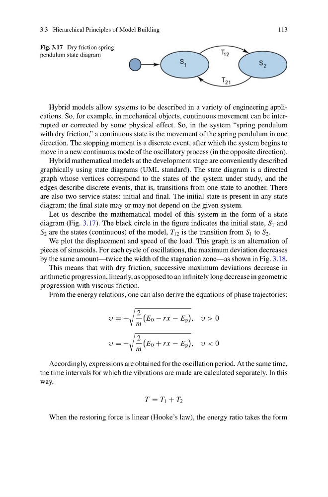
Fig. 3.17 Dry friction spring
pendulum state diagram
Hybrid models allow systems to be described in a variety of engineering applications. So, for example, in mechanical objects, continuous movement can be interrupted or corrected by some physical effect. So, in the system “spring pendulum
with dry friction,” a continuous state is the movement of the spring pendulum in one
direction. The stopping moment is a discrete event, after which the system begins to
move in a new continuous mode of the oscillatory process (in the opposite direction).
Hybrid mathematical models at the development stage are conveniently described
graphically using state diagrams (UML standard). The state diagram is a directed
graph whose vertices correspond to the states of the system under study, and the
edges describe discrete events, that is, transitions from one state to another. There
are also two service states: initial and final. The initial state is present in any state
diagram; the final state may or may not depend on the given system.
Let us describe the mathematical model of this system in the form of a state
diagram (Fig. 3.17). The black circle in the figure indicates the initial state, S 1 and
S 2 are the states (continuous) of the model, T 12 is the transition from S 1 to S 2 .
We plot the displacement and speed of the load. This graph is an alternation of
pieces of sinusoids. For each cycle of oscillations, the maximum deviation decreases
by the same amount—twice the width of the stagnation zone—as shown in Fig. 3.18.
This means that with dry friction, successive maximum deviations decrease in
arithmetic progression, linearly, as opposed to an infinitely long decrease in geometric
progression with viscous friction.
From the energy relations, one can also derive the equations of phase trajectories:
υ = +
2
m
E 0 − r x − E p
, υ > 0
υ = −
2
m
E 0 + r x − E p
, υ < 0
Accordingly, expressions are obtained for the oscillation period. At the same time,
the time intervals for which the vibrations are made are calculated separately. In this
way,
T = T 1 + T 2
When the restoring force is linear (Hooke’s law), the energy ratio takes the form
113
Fig. 3.17 Dry friction spring
pendulum state diagram
Hybrid models allow systems to be described in a variety of engineering applications. So, for example, in mechanical objects, continuous movement can be interrupted or corrected by some physical effect. So, in the system “spring pendulum
with dry friction,” a continuous state is the movement of the spring pendulum in one
direction. The stopping moment is a discrete event, after which the system begins to
move in a new continuous mode of the oscillatory process (in the opposite direction).
Hybrid mathematical models at the development stage are conveniently described
graphically using state diagrams (UML standard). The state diagram is a directed
graph whose vertices correspond to the states of the system under study, and the
edges describe discrete events, that is, transitions from one state to another. There
are also two service states: initial and final. The initial state is present in any state
diagram; the final state may or may not depend on the given system.
Let us describe the mathematical model of this system in the form of a state
diagram (Fig. 3.17). The black circle in the figure indicates the initial state, S 1 and
S 2 are the states (continuous) of the model, T 12 is the transition from S 1 to S 2 .
We plot the displacement and speed of the load. This graph is an alternation of
pieces of sinusoids. For each cycle of oscillations, the maximum deviation decreases
by the same amount—twice the width of the stagnation zone—as shown in Fig. 3.18.
This means that with dry friction, successive maximum deviations decrease in
arithmetic progression, linearly, as opposed to an infinitely long decrease in geometric
progression with viscous friction.
From the energy relations, one can also derive the equations of phase trajectories:
υ = +
2
m
E 0 − r x − E p
, υ > 0
υ = −
2
m
E 0 + r x − E p
, υ < 0
Accordingly, expressions are obtained for the oscillation period. At the same time,
the time intervals for which the vibrations are made are calculated separately. In this
way,
T = T 1 + T 2
When the restoring force is linear (Hooke’s law), the energy ratio takes the form