

228
M. Tsuji et.al.
Table 2 Tasks in the Block Gauss–Jordan workflow application. The input/output of the tasks
such as A i,j , B i,j , C i,j , · · · are blocks of a matrix
Task
Description
inversion(A i,j )
Compute the inversion of a block A i,j
prodMat(A i,j , B i,j )
Compute B i,j = A i,j B i,j
mProdMat(A i,j , B i,j ,C i,j )
Compute C i,j = −A i,j B i,j
prodDiff(A i,j , B i,j ,C i,j )
Compute C i,j = C i,j − A i,j B i,j
Table 3 # of blocks, block
sizes and # of tasks in the
Block Gauss–Jordan method
# of blocks 1 × 1
2 × 2
4 × 4 8 × 8 16 × 16
Block size 32,768 2 16,384 2 8192 2 4096 2 2048 2
# of tasks
3
18
108
696
4848
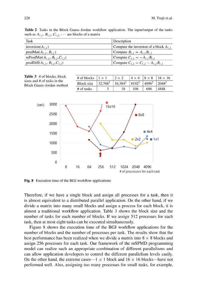
Fig. 8 Execution time of the BGJ workflow applications
Therefore, if we have a single block and assign all processes for a task, then it
is almost equivalent to a distributed parallel application. On the other hand, if we
divide a matrix into many small blocks and assign a process for each block, it is
almost a traditional workflow application. Table 3 shows the block size and the
number of tasks for each number of blocks. If we assign 512 processes for each
task, then at most eight tasks can be executed simultaneously.
Figure 8 shows the execution time of the BGJ workflow applications for the
number of blocks and the number of processes per task. The results show that the
best performance has been realized when we divide a matrix into 8 × 8 blocks and
assign 256 processes for each task. Our framework of the mSPMD programming
model can realize such an appropriate combination of different parallelisms and
can allow application developers to control the different parallelism levels easily.
On the other hand, the extreme cases—1 × 1 block and 16 × 16 blocks—have not
performed well. Also, assigning too many processes for small tasks, for example,
M. Tsuji et.al.
Table 2 Tasks in the Block Gauss–Jordan workflow application. The input/output of the tasks
such as A i,j , B i,j , C i,j , · · · are blocks of a matrix
Task
Description
inversion(A i,j )
Compute the inversion of a block A i,j
prodMat(A i,j , B i,j )
Compute B i,j = A i,j B i,j
mProdMat(A i,j , B i,j ,C i,j )
Compute C i,j = −A i,j B i,j
prodDiff(A i,j , B i,j ,C i,j )
Compute C i,j = C i,j − A i,j B i,j
Table 3 # of blocks, block
sizes and # of tasks in the
Block Gauss–Jordan method
# of blocks 1 × 1
2 × 2
4 × 4 8 × 8 16 × 16
Block size 32,768 2 16,384 2 8192 2 4096 2 2048 2
# of tasks
3
18
108
696
4848
Fig. 8 Execution time of the BGJ workflow applications
Therefore, if we have a single block and assign all processes for a task, then it
is almost equivalent to a distributed parallel application. On the other hand, if we
divide a matrix into many small blocks and assign a process for each block, it is
almost a traditional workflow application. Table 3 shows the block size and the
number of tasks for each number of blocks. If we assign 512 processes for each
task, then at most eight tasks can be executed simultaneously.
Figure 8 shows the execution time of the BGJ workflow applications for the
number of blocks and the number of processes per task. The results show that the
best performance has been realized when we divide a matrix into 8 × 8 blocks and
assign 256 processes for each task. Our framework of the mSPMD programming
model can realize such an appropriate combination of different parallelisms and
can allow application developers to control the different parallelism levels easily.
On the other hand, the extreme cases—1 × 1 block and 16 × 16 blocks—have not
performed well. Also, assigning too many processes for small tasks, for example,