

Hybrid-View Programming of Nuclear Fusion Simulation Code in XcalableMP
195
and particle dimensions exhibited good scalability, whereas scaling on the radial
dimension was poor. Figure 13 shows that the performance of decomposition on the
radial dimension decreased as the number of nodes increased compared with the
other two types of domain decomposition, as shown in Figs. 12 and 14. Most of the
communications are performed at the neighboring surface during decomposition on
any dimension and the total amount of communication data does not vary greatly;
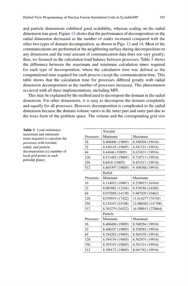
thus, we focused on the calculation load balance between processes. Table 5 shows
the difference between the maximum and minimum calculation times required
for each type of decomposition, where the calculation time was defined as the
computational time required for each process except the communication time. This
table shows that the calculation time for processes differed greatly with radial
dimension decomposition as the number of processes increased. This phenomenon
occurred with all three implementations, including MPI.
This may be explained by the method used to decompose the domain in the radial
dimension. For other dimensions, it is easy to decompose the domain completely
and equally for all processes. However, decomposition is complicated in the radial
dimension because the domain volume varies in the inner part and outer part due to
the torus form of the problem space. The volume and the corresponding grid size
Table 5 Load imbalance:
maximum and minimum
times required to calculate the
processes with toroidal,
radial, and particle
decomposition [s] (number of
local grid points in each
poloidal plane)
Toroidal
Processes Minimum
Maximum
16
8.408406 (19805) 8.548204 (19916)
32
8.440145 (19805) 8.541321 (19916)
64
8.44846 (19805)
8.631631 (19916)
128
8.511492 (19805) 8.718713 (19916)
256
8.6418 (19805)
8.853517 (19916)
512
8.865397 (19805) 9.109388 (19916)
Radial
Processes Minimum
Maximum
16
8.114932 (10967) 8.270015 (16164)
32
8.083982 (12104) 8.539186 (24200)
64
8.075058 (14130) 9.487029 (33462)
128
8.070919 (17422) 11.014277 (74745)
256
8.232447 (23198) 12.686402 (141700)
512
8.763279 (34522) 16.508915 (270844)
Particle
Processes Minimum
Maximum
16
8.408406 (19805) 8.548204 (19916)
32
8.406107 (19805) 8.558563 (19916)
64
8.394203 (19805) 8.565195 (19916)
128
8.394159 (19805) 8.562974 (19916)
256
8.393343 (19805) 8.591214 (19916)
512
8.390172 (19805) 8.641762 (19916)
195
and particle dimensions exhibited good scalability, whereas scaling on the radial
dimension was poor. Figure 13 shows that the performance of decomposition on the
radial dimension decreased as the number of nodes increased compared with the
other two types of domain decomposition, as shown in Figs. 12 and 14. Most of the
communications are performed at the neighboring surface during decomposition on
any dimension and the total amount of communication data does not vary greatly;
thus, we focused on the calculation load balance between processes. Table 5 shows
the difference between the maximum and minimum calculation times required
for each type of decomposition, where the calculation time was defined as the
computational time required for each process except the communication time. This
table shows that the calculation time for processes differed greatly with radial
dimension decomposition as the number of processes increased. This phenomenon
occurred with all three implementations, including MPI.
This may be explained by the method used to decompose the domain in the radial
dimension. For other dimensions, it is easy to decompose the domain completely
and equally for all processes. However, decomposition is complicated in the radial
dimension because the domain volume varies in the inner part and outer part due to
the torus form of the problem space. The volume and the corresponding grid size
Table 5 Load imbalance:
maximum and minimum
times required to calculate the
processes with toroidal,
radial, and particle
decomposition [s] (number of
local grid points in each
poloidal plane)
Toroidal
Processes Minimum
Maximum
16
8.408406 (19805) 8.548204 (19916)
32
8.440145 (19805) 8.541321 (19916)
64
8.44846 (19805)
8.631631 (19916)
128
8.511492 (19805) 8.718713 (19916)
256
8.6418 (19805)
8.853517 (19916)
512
8.865397 (19805) 9.109388 (19916)
Radial
Processes Minimum
Maximum
16
8.114932 (10967) 8.270015 (16164)
32
8.083982 (12104) 8.539186 (24200)
64
8.075058 (14130) 9.487029 (33462)
128
8.070919 (17422) 11.014277 (74745)
256
8.232447 (23198) 12.686402 (141700)
512
8.763279 (34522) 16.508915 (270844)
Particle
Processes Minimum
Maximum
16
8.408406 (19805) 8.548204 (19916)
32
8.406107 (19805) 8.558563 (19916)
64
8.394203 (19805) 8.565195 (19916)
128
8.394159 (19805) 8.562974 (19916)
256
8.393343 (19805) 8.591214 (19916)
512
8.390172 (19805) 8.641762 (19916)