

186
K. Tsugane et al.
radial direction
poloidal angle
radial interval
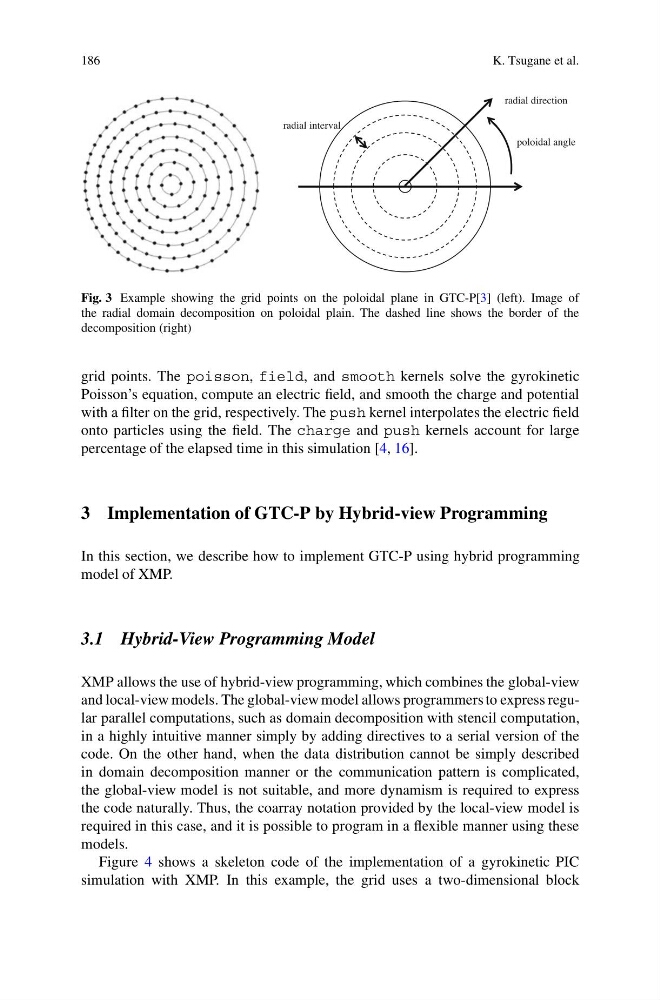
Fig. 3 Example showing the grid points on the poloidal plane in GTC-P[3] (left). Image of
the radial domain decomposition on poloidal plain. The dashed line shows the border of the
decomposition (right)
grid points. The poisson, field, and smooth kernels solve the gyrokinetic
Poisson’s equation, compute an electric field, and smooth the charge and potential
with a filter on the grid, respectively. The push kernel interpolates the electric field
onto particles using the field. The charge and push kernels account for large
percentage of the elapsed time in this simulation [4, 16].
3 Implementation of GTC-P by Hybrid-view Programming
In this section, we describe how to implement GTC-P using hybrid programming
model of XMP.
3.1 Hybrid-View Programming Model
XMP allows the use of hybrid-view programming, which combines the global-view
and local-view models. The global-view model allows programmers to express regular parallel computations, such as domain decomposition with stencil computation,
in a highly intuitive manner simply by adding directives to a serial version of the
code. On the other hand, when the data distribution cannot be simply described
in domain decomposition manner or the communication pattern is complicated,
the global-view model is not suitable, and more dynamism is required to express
the code naturally. Thus, the coarray notation provided by the local-view model is
required in this case, and it is possible to program in a flexible manner using these
models.
Figure 4 shows a skeleton code of the implementation of a gyrokinetic PIC
simulation with XMP. In this example, the grid uses a two-dimensional block
K. Tsugane et al.
radial direction
poloidal angle
radial interval
Fig. 3 Example showing the grid points on the poloidal plane in GTC-P[3] (left). Image of
the radial domain decomposition on poloidal plain. The dashed line shows the border of the
decomposition (right)
grid points. The poisson, field, and smooth kernels solve the gyrokinetic
Poisson’s equation, compute an electric field, and smooth the charge and potential
with a filter on the grid, respectively. The push kernel interpolates the electric field
onto particles using the field. The charge and push kernels account for large
percentage of the elapsed time in this simulation [4, 16].
3 Implementation of GTC-P by Hybrid-view Programming
In this section, we describe how to implement GTC-P using hybrid programming
model of XMP.
3.1 Hybrid-View Programming Model
XMP allows the use of hybrid-view programming, which combines the global-view
and local-view models. The global-view model allows programmers to express regular parallel computations, such as domain decomposition with stencil computation,
in a highly intuitive manner simply by adding directives to a serial version of the
code. On the other hand, when the data distribution cannot be simply described
in domain decomposition manner or the communication pattern is complicated,
the global-view model is not suitable, and more dynamism is required to express
the code naturally. Thus, the coarray notation provided by the local-view model is
required in this case, and it is possible to program in a flexible manner using these
models.
Figure 4 shows a skeleton code of the implementation of a gyrokinetic PIC
simulation with XMP. In this example, the grid uses a two-dimensional block