

160
M. Nakao
1 #pragma xmp template t[:]
2 #pragma xmp nodes p[*]
3 #pragma xmp distribute t[block] onto p
4
5 void xmp_graphgolf(int *edge)
6 {
7
:
8 int vertices = edge[0];
9 #pragma xmp template_fix t[vertices]
10 #pragma xmp loop on t[i]
11
for(int i=0;i
: // Calculate diameter and ASPL
13
}
14 #pragma xmp reduction(+:ASPL)
15 #pragma xmp reduction(max:diameter)
16
:
17 }
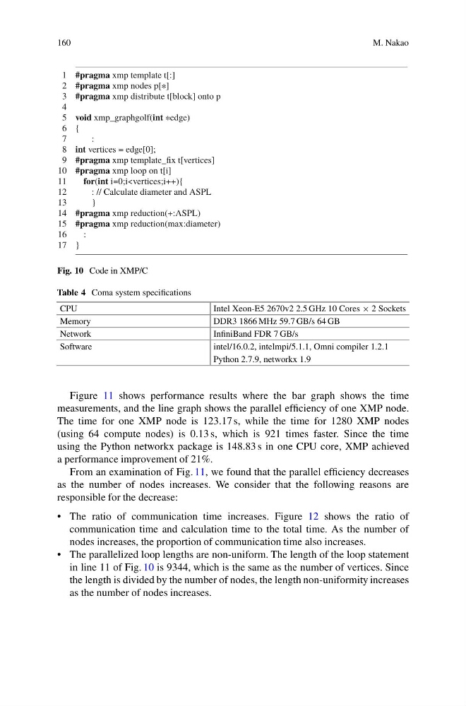
Fig. 10 Code in XMP/C
Table 4 Coma system specifications
CPU
Intel Xeon-E5 2670v2 2.5 GHz 10 Cores × 2 Sockets
Memory
DDR3 1866 MHz 59.7 GB/s 64 GB
Network
InfiniBand FDR 7 GB/s
Software
intel/16.0.2, intelmpi/5.1.1, Omni compiler 1.2.1
Python 2.7.9, networkx 1.9
Figure 11 shows performance results where the bar graph shows the time
measurements, and the line graph shows the parallel efficiency of one XMP node.
The time for one XMP node is 123.17 s, while the time for 1280 XMP nodes
(using 64 compute nodes) is 0.13 s, which is 921 times faster. Since the time
using the Python networkx package is 148.83 s in one CPU core, XMP achieved
a performance improvement of 21%.
From an examination of Fig. 11, we found that the parallel efficiency decreases
as the number of nodes increases. We consider that the following reasons are
responsible for the decrease:
• The ratio of communication time increases. Figure 12 shows the ratio of
communication time and calculation time to the total time. As the number of
nodes increases, the proportion of communication time also increases.
• The parallelized loop lengths are non-uniform. The length of the loop statement
in line 11 of Fig. 10 is 9344, which is the same as the number of vertices. Since
the length is divided by the number of nodes, the length non-uniformity increases
as the number of nodes increases.
M. Nakao
1 #pragma xmp template t[:]
2 #pragma xmp nodes p[*]
3 #pragma xmp distribute t[block] onto p
4
5 void xmp_graphgolf(int *edge)
6 {
7
:
8 int vertices = edge[0];
9 #pragma xmp template_fix t[vertices]
10 #pragma xmp loop on t[i]
11
for(int i=0;i
: // Calculate diameter and ASPL
13
}
14 #pragma xmp reduction(+:ASPL)
15 #pragma xmp reduction(max:diameter)
16
:
17 }
Fig. 10 Code in XMP/C
Table 4 Coma system specifications
CPU
Intel Xeon-E5 2670v2 2.5 GHz 10 Cores × 2 Sockets
Memory
DDR3 1866 MHz 59.7 GB/s 64 GB
Network
InfiniBand FDR 7 GB/s
Software
intel/16.0.2, intelmpi/5.1.1, Omni compiler 1.2.1
Python 2.7.9, networkx 1.9
Figure 11 shows performance results where the bar graph shows the time
measurements, and the line graph shows the parallel efficiency of one XMP node.
The time for one XMP node is 123.17 s, while the time for 1280 XMP nodes
(using 64 compute nodes) is 0.13 s, which is 921 times faster. Since the time
using the Python networkx package is 148.83 s in one CPU core, XMP achieved
a performance improvement of 21%.
From an examination of Fig. 11, we found that the parallel efficiency decreases
as the number of nodes increases. We consider that the following reasons are
responsible for the decrease:
• The ratio of communication time increases. Figure 12 shows the ratio of
communication time and calculation time to the total time. As the number of
nodes increases, the proportion of communication time also increases.
• The parallelized loop lengths are non-uniform. The length of the loop statement
in line 11 of Fig. 10 is 9344, which is the same as the number of vertices. Since
the length is divided by the number of nodes, the length non-uniformity increases
as the number of nodes increases.