

from input/output—input files; from spectrum processing—
select spectra, align retention times; from compound detection—detect compounds, group compounds, fill gaps; from
peak area refinement—normalize areas, mark background
compounds; from compound identification—predict compositions, search mzCloud, assign compound annotations, search
ChemSpider, search mzVault; from pathway mapping—map to
KEGG pathways, map to metabolika pathways; from compound scoring—apply mzLogic; from post-processing—differential analysis, descriptive statistics.
3. After adding the processing workflow, you will add new files to
the study. Here you must indicate study factors (for example
control and treatment). Study factors can be categorical,
numerical, or biological replicates. You must characterize each
of the new files that you add to your study by selecting sample
types and assigning study factor values to each file.
4. Next you will set up sample groups and ratios for a new analysis.
For example, in our study we had three replicates of control and
three of treated. We grouped these files and created ratios of
treated/control.
5. Finally, submit your new study to the job queue to run. After
the run is completed, the results can be viewed and analyzed in
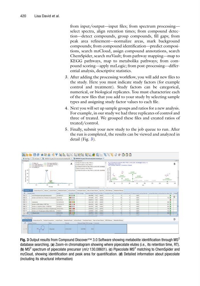
detail (Fig. 3).
Fig. 3 Output results from Compound Discover™ 3.0 Software showing metabolite identification through MS
2
database searching. (a) Zoom-in chromatogram showing where pipecolate elutes (i.e., its retention time, RT).
(b) MS
2
spectrum of pipecolate precursor (m/z 130.08601). (c) Pipecolate MS
2
matching to ChemSpider and
mzCloud, showing identification and peak area for quantification. (d) Detailed information about pipecolate
(including its structural information)
420
Lisa David et al.
select spectra, align retention times; from compound detection—detect compounds, group compounds, fill gaps; from
peak area refinement—normalize areas, mark background
compounds; from compound identification—predict compositions, search mzCloud, assign compound annotations, search
ChemSpider, search mzVault; from pathway mapping—map to
KEGG pathways, map to metabolika pathways; from compound scoring—apply mzLogic; from post-processing—differential analysis, descriptive statistics.
3. After adding the processing workflow, you will add new files to
the study. Here you must indicate study factors (for example
control and treatment). Study factors can be categorical,
numerical, or biological replicates. You must characterize each
of the new files that you add to your study by selecting sample
types and assigning study factor values to each file.
4. Next you will set up sample groups and ratios for a new analysis.
For example, in our study we had three replicates of control and
three of treated. We grouped these files and created ratios of
treated/control.
5. Finally, submit your new study to the job queue to run. After
the run is completed, the results can be viewed and analyzed in
detail (Fig. 3).
Fig. 3 Output results from Compound Discover™ 3.0 Software showing metabolite identification through MS
2
database searching. (a) Zoom-in chromatogram showing where pipecolate elutes (i.e., its retention time, RT).
(b) MS
2
spectrum of pipecolate precursor (m/z 130.08601). (c) Pipecolate MS
2
matching to ChemSpider and
mzCloud, showing identification and peak area for quantification. (d) Detailed information about pipecolate
(including its structural information)
420
Lisa David et al.