

Optimal FF SFs are obtained from minimization of the LSMF, Eq. (2.29), for a
given training set of molecules. In this case, the LSMF is non-quadratic in contrast
to US procedure and has to be minimized iteratively using, e.g., Newton–Raphson
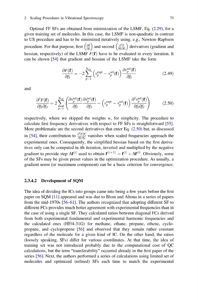
procedure. For that purpose, first
@F
@f I
and second
@
2 F
@f I @f J
derivatives (gradient and
hessian, respectively) of the LSMF F f
ð Þ have to be evaluated in every iteration. It
can be shown [54] that gradient and hessian of the LSMF take the form
@F f
ð Þ
@f I
¼ À2
X N vib
p¼1
m
expt
p
À m
scl
p f
ð Þ
@m
scl
p f
ð Þ
@f I
ð2:49Þ
and
@
2 F f
ð Þ
@f I @f J
¼ 2
X N vib
p¼1
@m
scl
p f
ð Þ
@f I
@m
scl
p f
ð Þ
@f J
À m
expt
p
À m
scl
p f
ð Þ
@
2 m
scl
p f
ð Þ
@f I @f J
!
ð2:50Þ
respectively, where we skipped the weights w, for simplicity. The procedure to
calculate first frequency derivatives with respect to FF SFs is straightforward [55].
More problematic are the second derivatives that enter Eq. (2.50) but, as discussed
in [54], their contribution to
@
2 F f
ð Þ
@f I @f J
vanishes when scaled frequencies approach the
experimental ones. Consequently, the simplified hessian based on the first derivatives only can be computed in ith iteration, inverted and multiplied by the negative
gradient to provide step Df
i
ð Þ used to obtain f
i þ 1
ð
Þ
¼ f
i
ð Þ
þ Df
i
ð Þ . Obviously, some
of the SFs may be given preset values in the optimization procedure. As usually, a
gradient norm (or maximum component) can be a basic criterion for convergence.
2.3.4.2 Development of SQM
The idea of dividing the ICs into groups came into being a few years before the first
paper on SQM [11] appeared and was due to Blom and Altona in a series of papers
from the mid-1970s [56–61]. The authors recognized that adopting different SF to
different FCs provides much better agreement with experimental frequencies than in
the case of using a single SF. They calculated ratios between diagonal FCs derived
from both experimental fundamental and experimental harmonic frequencies and
the calculated ones (HF/4-31G) for methane, ethane, propane, ethene, cyclopropane, and cyclopropene [56] and observed that they remain rather constant
regardless of the molecule for a given kind of IC. On the other hand, the ratios
(loosely speaking, SFs) differ for various coordinates. At that time, the idea of
training set was not introduced probably due to the computational cost of QC
calculations, but the term “transferability” occurred already in the first paper of the
series [56]. Next, the authors performed a series of calculations using limited set of
molecules and optimized (refined) SFs each time to match the experimental
2 Scaling Procedures in Vibrational Spectroscopy
75
given training set of molecules. In this case, the LSMF is non-quadratic in contrast
to US procedure and has to be minimized iteratively using, e.g., Newton–Raphson
procedure. For that purpose, first
@F
@f I
and second
@
2 F
@f I @f J
derivatives (gradient and
hessian, respectively) of the LSMF F f
ð Þ have to be evaluated in every iteration. It
can be shown [54] that gradient and hessian of the LSMF take the form
@F f
ð Þ
@f I
¼ À2
X N vib
p¼1
m
expt
p
À m
scl
p f
ð Þ
@m
scl
p f
ð Þ
@f I
ð2:49Þ
and
@
2 F f
ð Þ
@f I @f J
¼ 2
X N vib
p¼1
@m
scl
p f
ð Þ
@f I
@m
scl
p f
ð Þ
@f J
À m
expt
p
À m
scl
p f
ð Þ
@
2 m
scl
p f
ð Þ
@f I @f J
!
ð2:50Þ
respectively, where we skipped the weights w, for simplicity. The procedure to
calculate first frequency derivatives with respect to FF SFs is straightforward [55].
More problematic are the second derivatives that enter Eq. (2.50) but, as discussed
in [54], their contribution to
@
2 F f
ð Þ
@f I @f J
vanishes when scaled frequencies approach the
experimental ones. Consequently, the simplified hessian based on the first derivatives only can be computed in ith iteration, inverted and multiplied by the negative
gradient to provide step Df
i
ð Þ used to obtain f
i þ 1
ð
Þ
¼ f
i
ð Þ
þ Df
i
ð Þ . Obviously, some
of the SFs may be given preset values in the optimization procedure. As usually, a
gradient norm (or maximum component) can be a basic criterion for convergence.
2.3.4.2 Development of SQM
The idea of dividing the ICs into groups came into being a few years before the first
paper on SQM [11] appeared and was due to Blom and Altona in a series of papers
from the mid-1970s [56–61]. The authors recognized that adopting different SF to
different FCs provides much better agreement with experimental frequencies than in
the case of using a single SF. They calculated ratios between diagonal FCs derived
from both experimental fundamental and experimental harmonic frequencies and
the calculated ones (HF/4-31G) for methane, ethane, propane, ethene, cyclopropane, and cyclopropene [56] and observed that they remain rather constant
regardless of the molecule for a given kind of IC. On the other hand, the ratios
(loosely speaking, SFs) differ for various coordinates. At that time, the idea of
training set was not introduced probably due to the computational cost of QC
calculations, but the term “transferability” occurred already in the first paper of the
series [56]. Next, the authors performed a series of calculations using limited set of
molecules and optimized (refined) SFs each time to match the experimental
2 Scaling Procedures in Vibrational Spectroscopy
75