

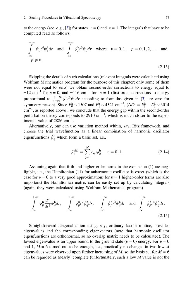
to the energy (see, e.g., [3]) for states t = 0 and t = 1. The integrals that have to be
computed read as follows:
Z þ 1
À1
w
h
t r
4 w
h
t dr and
Z þ 1
À1
w
h
p r
3 w
h
t dr where t ¼ 0; 1; p ¼ 0; 1; 2; . . . and
p 6 ¼ t:
ð2:13Þ
Skipping the details of such calculations (relevant integrals were calculated using
Wolfram Mathematica program for the purpose of this chapter; only some of them
were not equal to zero) we obtain second-order corrections to energy equal to
−12 cm
−1 for t = 0, and −116 cm
−1 for t = 1 (first-order corrections to energy
proportional to
R þ 1
À1 w
h
t r
3 w
h
t dr according to formulas given in [3] are zero for
symmetry reason). Since E
h
0 $ 1507 and E
h
1 $ 4521 cm
−1 , (DE
h
¼ E
h
1 À E
h
0 $ 3014
cm
−1 , as reported above), we conclude that the energy gap within the second-order
perturbation theory corresponds to 2910 cm
−1 , which is much closer to the experimental value of 2886 cm
−1 .
Alternatively, one can use variation method within, say, Ritz framework, and
choose the trial wavefunction as a linear combination of harmonic oscillator
eigenfunctions w
h
q which form a basis set, i.e.,
w
trial
t
¼
X M
q¼0
c qt w
h
q ; t ¼ 0; 1:
ð2:14Þ
Assuming again that fifth and higher-order terms in the expansion (1) are negligible, i.e., the Hamiltonian (11) for anharmonic oscillator is exact (which is the
case for t = 0 to a very good approximation; for t = 1 higher-order terms are also
important) the Hamiltonian matrix can be easily set up by calculating integrals
(again, they were calculated using Wolfram Mathematica program)
Z þ 1
À1
w
h
p
d
2
dr 2 w
h
q dr;
Z þ 1
À1
w
h
p r
2 w
h
q dr;
Z þ 1
À1
w
h
p r
3 w
h
q dr and
Z þ 1
À1
w
h
p r
4 w
h
q dr:
ð2:15Þ
Straightforward diagonalization using, say, ordinary Jacobi routine, provides
eigenvalues and the corresponding eigenvectors (note that harmonic oscillator
eigenfunctions are orthonormal, so no overlap matrix needs to be calculated). The
lowest eigenvalue is an upper bound to the ground state (t = 0) energy. For t = 0
and 1, M = 6 turned out to be enough, i.e., practically no changes in two lowest
eigenvalues were observed upon further increasing of M, so the basis set for M = 6
can be regarded as (nearly) complete (unfortunately, such a low M value is not the
2 Scaling Procedures in Vibrational Spectroscopy
57
computed read as follows:
Z þ 1
À1
w
h
t r
4 w
h
t dr and
Z þ 1
À1
w
h
p r
3 w
h
t dr where t ¼ 0; 1; p ¼ 0; 1; 2; . . . and
p 6 ¼ t:
ð2:13Þ
Skipping the details of such calculations (relevant integrals were calculated using
Wolfram Mathematica program for the purpose of this chapter; only some of them
were not equal to zero) we obtain second-order corrections to energy equal to
−12 cm
−1 for t = 0, and −116 cm
−1 for t = 1 (first-order corrections to energy
proportional to
R þ 1
À1 w
h
t r
3 w
h
t dr according to formulas given in [3] are zero for
symmetry reason). Since E
h
0 $ 1507 and E
h
1 $ 4521 cm
−1 , (DE
h
¼ E
h
1 À E
h
0 $ 3014
cm
−1 , as reported above), we conclude that the energy gap within the second-order
perturbation theory corresponds to 2910 cm
−1 , which is much closer to the experimental value of 2886 cm
−1 .
Alternatively, one can use variation method within, say, Ritz framework, and
choose the trial wavefunction as a linear combination of harmonic oscillator
eigenfunctions w
h
q which form a basis set, i.e.,
w
trial
t
¼
X M
q¼0
c qt w
h
q ; t ¼ 0; 1:
ð2:14Þ
Assuming again that fifth and higher-order terms in the expansion (1) are negligible, i.e., the Hamiltonian (11) for anharmonic oscillator is exact (which is the
case for t = 0 to a very good approximation; for t = 1 higher-order terms are also
important) the Hamiltonian matrix can be easily set up by calculating integrals
(again, they were calculated using Wolfram Mathematica program)
Z þ 1
À1
w
h
p
d
2
dr 2 w
h
q dr;
Z þ 1
À1
w
h
p r
2 w
h
q dr;
Z þ 1
À1
w
h
p r
3 w
h
q dr and
Z þ 1
À1
w
h
p r
4 w
h
q dr:
ð2:15Þ
Straightforward diagonalization using, say, ordinary Jacobi routine, provides
eigenvalues and the corresponding eigenvectors (note that harmonic oscillator
eigenfunctions are orthonormal, so no overlap matrix needs to be calculated). The
lowest eigenvalue is an upper bound to the ground state (t = 0) energy. For t = 0
and 1, M = 6 turned out to be enough, i.e., practically no changes in two lowest
eigenvalues were observed upon further increasing of M, so the basis set for M = 6
can be regarded as (nearly) complete (unfortunately, such a low M value is not the
2 Scaling Procedures in Vibrational Spectroscopy
57