possible results (measurement problem, collapse of the wave function), which
culminates in the formulation of the equation describing the evolution of the state of
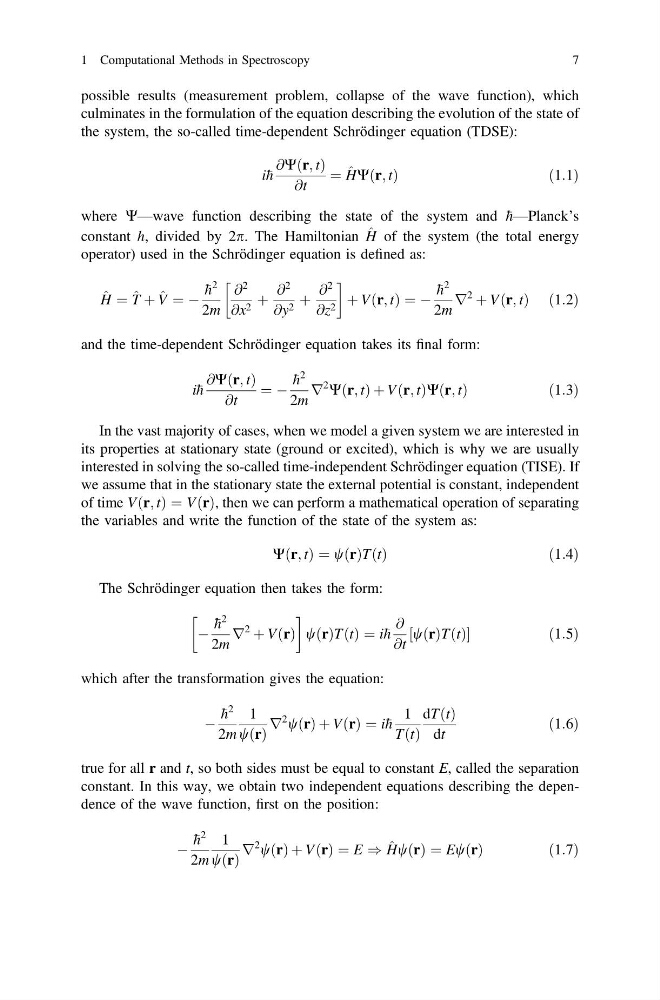
the system, the so-called time-dependent Schrödinger equation (TDSE):
i h
@Wðr; tÞ
@t
¼ ^
HWðr; tÞ
ð 1:1Þ
where W—wave function describing the state of the system and h—Planck’s
constant h, divided by 2p. The Hamiltonian ^
H of the system (the total energy
operator) used in the Schrödinger equation is defined as:
^
H ¼ ^
T þ ^
V ¼ À
h
2
2m
@
2
@x 2 þ
@
2
@y 2 þ
@
2
@z 2
!
þ Vðr; tÞ ¼ À
h
2
2m
r
2
þ Vðr; tÞ ð1:2Þ
and the time-dependent Schrödinger equation takes its final form:
i h
@W r; t
ð Þ
@t
¼ À
h
2
2m
r
2
W r; t
ð ÞþV r; t
ð ÞW r; t
ð Þ
ð1:3Þ
In the vast majority of cases, when we model a given system we are interested in
its properties at stationary state (ground or excited), which is why we are usually
interested in solving the so-called time-independent Schrödinger equation (TISE). If
we assume that in the stationary state the external potential is constant, independent
of time V r; t
ð Þ ¼ VðrÞ, then we can perform a mathematical operation of separating
the variables and write the function of the state of the system as:
Wðr; tÞ ¼ wðrÞTðtÞ
ð 1:4Þ
The Schrödinger equation then takes the form:
À
h
2
2m
r
2
þ VðrÞ
!
wðrÞTðtÞ ¼ i h
@
@t
½wðrÞTðtފ
ð1:5Þ
which after the transformation gives the equation:
À
h
2
2m
1
wðrÞ
r
2 wðrÞ þ VðrÞ ¼ i h
1
TðtÞ
dTðtÞ
dt
ð1:6Þ
true for all r and t, so both sides must be equal to constant E, called the separation
constant. In this way, we obtain two independent equations describing the dependence of the wave function, first on the position:
À
h
2
2m
1
wðrÞ
r
2 wðrÞ þ VðrÞ ¼ E ) ^
HwðrÞ ¼ EwðrÞ
ð 1:7Þ
1 Computational Methods in Spectroscopy
7