

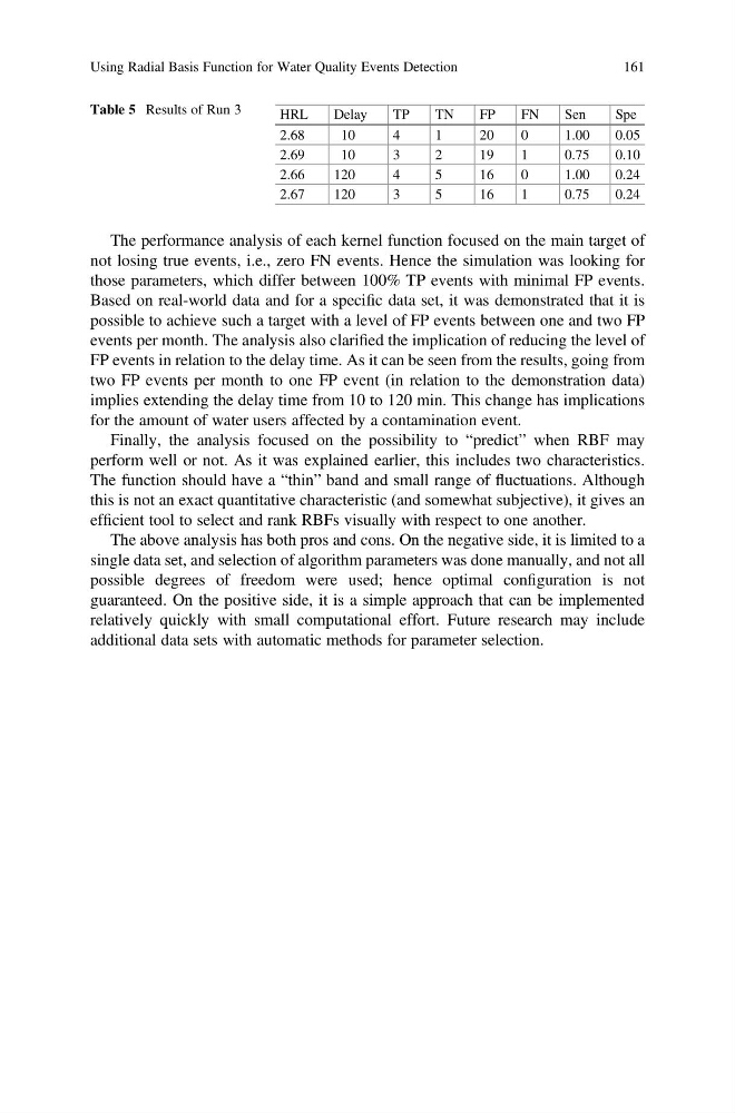
The performance analysis of each kernel function focused on the main target of
not losing true events, i.e., zero FN events. Hence the simulation was looking for
those parameters, which differ between 100% TP events with minimal FP events.
Based on real-world data and for a specific data set, it was demonstrated that it is
possible to achieve such a target with a level of FP events between one and two FP
events per month. The analysis also clarified the implication of reducing the level of
FP events in relation to the delay time. As it can be seen from the results, going from
two FP events per month to one FP event (in relation to the demonstration data)
implies extending the delay time from 10 to 120 min. This change has implications
for the amount of water users affected by a contamination event.
Finally, the analysis focused on the possibility to “predict” when RBF may
perform well or not. As it was explained earlier, this includes two characteristics.
The function should have a “thin” band and small range of fluctuations. Although
this is not an exact quantitative characteristic (and somewhat subjective), it gives an
efficient tool to select and rank RBFs visually with respect to one another.
The above analysis has both pros and cons. On the negative side, it is limited to a
single data set, and selection of algorithm parameters was done manually, and not all
possible degrees of freedom were used; hence optimal configuration is not
guaranteed. On the positive side, it is a simple approach that can be implemented
relatively quickly with small computational effort. Future research may include
additional data sets with automatic methods for parameter selection.
Table 5 Results of Run 3
HRL
Delay
TP
TN
FP
FN
Sen
Spe
2.68
10
4
1
20
0
1.00
0.05
2.69
10
3
2
19
1
0.75
0.10
2.66
120
4
5
16
0
1.00
0.24
2.67
120
3
5
16
1
0.75
0.24
Using Radial Basis Function for Water Quality Events Detection
161
not losing true events, i.e., zero FN events. Hence the simulation was looking for
those parameters, which differ between 100% TP events with minimal FP events.
Based on real-world data and for a specific data set, it was demonstrated that it is
possible to achieve such a target with a level of FP events between one and two FP
events per month. The analysis also clarified the implication of reducing the level of
FP events in relation to the delay time. As it can be seen from the results, going from
two FP events per month to one FP event (in relation to the demonstration data)
implies extending the delay time from 10 to 120 min. This change has implications
for the amount of water users affected by a contamination event.
Finally, the analysis focused on the possibility to “predict” when RBF may
perform well or not. As it was explained earlier, this includes two characteristics.
The function should have a “thin” band and small range of fluctuations. Although
this is not an exact quantitative characteristic (and somewhat subjective), it gives an
efficient tool to select and rank RBFs visually with respect to one another.
The above analysis has both pros and cons. On the negative side, it is limited to a
single data set, and selection of algorithm parameters was done manually, and not all
possible degrees of freedom were used; hence optimal configuration is not
guaranteed. On the positive side, it is a simple approach that can be implemented
relatively quickly with small computational effort. Future research may include
additional data sets with automatic methods for parameter selection.
Table 5 Results of Run 3
HRL
Delay
TP
TN
FP
FN
Sen
Spe
2.68
10
4
1
20
0
1.00
0.05
2.69
10
3
2
19
1
0.75
0.10
2.66
120
4
5
16
0
1.00
0.24
2.67
120
3
5
16
1
0.75
0.24
Using Radial Basis Function for Water Quality Events Detection
161