

can be seen from Fig. 11, the noise of this function is relatively small. This can be
seen from the red arrows in Fig. 11.
The last results of Run 4 are shown in Fig. 12 and Table 6.
This function performs better than the other runs. As it can be seen from Table 6,
by choosing HRL between 2.82 and 2.83, it is possible to reduce the number of FP
events from 20 to 13 with a cost of a single FN event without increasing the
delay time.
One may ask at this point, what differs the four functions one from the other, and
is it possible just to be looking at the RBF chart to “predict” which RBF will perform
well and which will not? A closer look at Figs. 3, 4, 5, and 6 may reveal the
“patterns” of good functions and “bad” functions. Function 2, which had the worst
performance, has a relatively wide “blue band.” This band is marked with red arrows
in Figs. 4 and 5. And as it can be seen, the band of function 2 is bigger. A bigger band
makes it difficult to observe when a sample leaves the normal zone for the abnormal
zone. A second characteristic, which differs good from bad functions, is the size of
the range where fluctuation of the RBF is located. Comparing Figs. 3, 4, 5, and 6,
one may observe that in Fig. 9 the majority of RBF values are located between 2.6
and 2.72 (see green arrow in Fig. 9). However, in Fig. 12 the majority is between
values 2.8 and 2.86 (see green arrow as Fig. 12). Hence the range of fluctuations in
Fig. 9 is twice as big as the range in Fig. 12. This gives the second criteria for
different RBFs in the vertical axis.
The smaller the range of fluctuations, the easier it is to detect abnormality.
7 Concluding Remarks
This chapter has demonstrated one approach of how RBF can be used to classify
abnormal events in water supply systems directly from manually tagged sensor data.
The methodology is based on prior (manual) classification of events into true and
false events. Once enough true events exist, the set of these events may be used as a
training set. From this stage a second set of events (which contains true and false) are
used for the calibration of the RBF algorithm. The parameters of the algorithm
include the value of the RBF, which is used as a threshold, and the delay time before
an alert is declared. As it was explained early, for the sake of simplicity, the
additional parameters of the RBF have been kept fixed in the current analysis with
a value of 1.
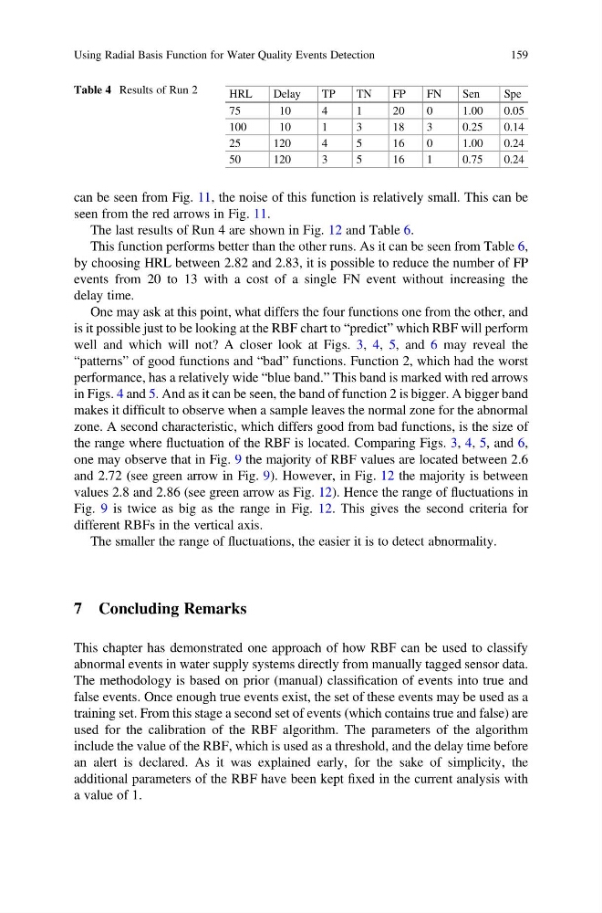
Table 4 Results of Run 2
HRL
Delay
TP
TN
FP
FN
Sen
Spe
75
10
4
1
20
0
1.00
0.05
100
10
1
3
18
3
0.25
0.14
25
120
4
5
16
0
1.00
0.24
50
120
3
5
16
1
0.75
0.24
Using Radial Basis Function for Water Quality Events Detection
159
seen from the red arrows in Fig. 11.
The last results of Run 4 are shown in Fig. 12 and Table 6.
This function performs better than the other runs. As it can be seen from Table 6,
by choosing HRL between 2.82 and 2.83, it is possible to reduce the number of FP
events from 20 to 13 with a cost of a single FN event without increasing the
delay time.
One may ask at this point, what differs the four functions one from the other, and
is it possible just to be looking at the RBF chart to “predict” which RBF will perform
well and which will not? A closer look at Figs. 3, 4, 5, and 6 may reveal the
“patterns” of good functions and “bad” functions. Function 2, which had the worst
performance, has a relatively wide “blue band.” This band is marked with red arrows
in Figs. 4 and 5. And as it can be seen, the band of function 2 is bigger. A bigger band
makes it difficult to observe when a sample leaves the normal zone for the abnormal
zone. A second characteristic, which differs good from bad functions, is the size of
the range where fluctuation of the RBF is located. Comparing Figs. 3, 4, 5, and 6,
one may observe that in Fig. 9 the majority of RBF values are located between 2.6
and 2.72 (see green arrow in Fig. 9). However, in Fig. 12 the majority is between
values 2.8 and 2.86 (see green arrow as Fig. 12). Hence the range of fluctuations in
Fig. 9 is twice as big as the range in Fig. 12. This gives the second criteria for
different RBFs in the vertical axis.
The smaller the range of fluctuations, the easier it is to detect abnormality.
7 Concluding Remarks
This chapter has demonstrated one approach of how RBF can be used to classify
abnormal events in water supply systems directly from manually tagged sensor data.
The methodology is based on prior (manual) classification of events into true and
false events. Once enough true events exist, the set of these events may be used as a
training set. From this stage a second set of events (which contains true and false) are
used for the calibration of the RBF algorithm. The parameters of the algorithm
include the value of the RBF, which is used as a threshold, and the delay time before
an alert is declared. As it was explained early, for the sake of simplicity, the
additional parameters of the RBF have been kept fixed in the current analysis with
a value of 1.
Table 4 Results of Run 2
HRL
Delay
TP
TN
FP
FN
Sen
Spe
75
10
4
1
20
0
1.00
0.05
100
10
1
3
18
3
0.25
0.14
25
120
4
5
16
0
1.00
0.24
50
120
3
5
16
1
0.75
0.24
Using Radial Basis Function for Water Quality Events Detection
159