

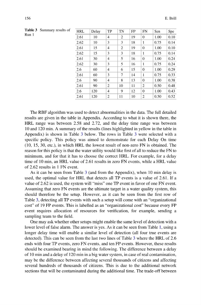
The RBF algorithm was used to detect abnormalities in the data. The full detailed
results are given in the table in Appendix. According to what it is shown there, the
HRL range was between 2.58 and 2.72, and the delay time range was between
10 and 120 min. A summary of the results (lines highlighted in yellow in the table in
Appendix) is shown in Table 3 below. The rows in Table 3 were selected with a
specific policy. This policy was aimed to demonstrate for each Delay On time
(10, 15, 30, etc.), in which HRL the lowest result of non-zero FN is obtained. The
reason for this policy is that the water utility would like first of all to reduce the FN to
minimum, and for that it has to choose the correct HRL. For example, for a delay
time of 10 min, an HRL value of 2.61 results in zero FN events, while a HRL value
of 2.62 results in 1 FN event.
As it can be seen from Table 3 (and from the Appendix), when 10 min delay is
used, the optimal value for HRL that detects all TP events is a value of 2.61. If a
value of 2.62 is used, the system will “miss” one TP event in favor of one FN event.
Assuming that zero FN events are the ultimate target in a water quality system, this
should therefore be the setup. However, as it can be seen from the first row of
Table 3, detecting all TP events with such a setup will come with an “organizational
cost” of 19 FP events. This is labelled as an “organizational cost” because every FP
event requires allocation of resources for verification, for example, sending a
sampling team to the field.
One may ask whether other setups might enable the same level of detection with a
lower level of false alarm. The answer is yes. As it can be seen from Table 1, using a
longer delay time will enable a similar level of detection (all four true events are
detected). This can be seen from the last two lines of Table 3 where the HRL of 2.6
ends with four TP events, zero FN events, and ten FP events. However, these results
should be examined bearing in mind the following. The difference between a delay
of 10 min and a delay of 120 min in a big water system, in case of real contamination,
may be the difference between affecting several thousands of citizens and affecting
several hundreds of thousands of citizens. This is due to the additional network
sections that will be contaminated during the additional time. The trade-off between
Table 3 Summary results of
Run 1
HRL
Delay
TP
TN
FP
FN
Sen
Spe
2.61
10
4
2
19
0
1.00
0.10
2.62
10
3
3
18
1
0.75
0.14
2.61
15
4
2
19
0
1.00
0.10
2.62
15
3
3
18
1
0.75
0.14
2.61
30
4
5
16
0
1.00
0.24
2.62
30
3
5
16
1
0.75
0.24
2.6
60
4
6
15
0
1.00
0.29
2.61
60
3
7
14
1
0.75
0.33
2.6
90
4
8
13
0
1.00
0.38
2.61
90
2
10
11
2
0.50
0.48
2.6
120
4
9
12
0
1.00
0.43
2.61
120
2
11
10
2
0.50
0.52
156
E. Brill
results are given in the table in Appendix. According to what it is shown there, the
HRL range was between 2.58 and 2.72, and the delay time range was between
10 and 120 min. A summary of the results (lines highlighted in yellow in the table in
Appendix) is shown in Table 3 below. The rows in Table 3 were selected with a
specific policy. This policy was aimed to demonstrate for each Delay On time
(10, 15, 30, etc.), in which HRL the lowest result of non-zero FN is obtained. The
reason for this policy is that the water utility would like first of all to reduce the FN to
minimum, and for that it has to choose the correct HRL. For example, for a delay
time of 10 min, an HRL value of 2.61 results in zero FN events, while a HRL value
of 2.62 results in 1 FN event.
As it can be seen from Table 3 (and from the Appendix), when 10 min delay is
used, the optimal value for HRL that detects all TP events is a value of 2.61. If a
value of 2.62 is used, the system will “miss” one TP event in favor of one FN event.
Assuming that zero FN events are the ultimate target in a water quality system, this
should therefore be the setup. However, as it can be seen from the first row of
Table 3, detecting all TP events with such a setup will come with an “organizational
cost” of 19 FP events. This is labelled as an “organizational cost” because every FP
event requires allocation of resources for verification, for example, sending a
sampling team to the field.
One may ask whether other setups might enable the same level of detection with a
lower level of false alarm. The answer is yes. As it can be seen from Table 1, using a
longer delay time will enable a similar level of detection (all four true events are
detected). This can be seen from the last two lines of Table 3 where the HRL of 2.6
ends with four TP events, zero FN events, and ten FP events. However, these results
should be examined bearing in mind the following. The difference between a delay
of 10 min and a delay of 120 min in a big water system, in case of real contamination,
may be the difference between affecting several thousands of citizens and affecting
several hundreds of thousands of citizens. This is due to the additional network
sections that will be contaminated during the additional time. The trade-off between
Table 3 Summary results of
Run 1
HRL
Delay
TP
TN
FP
FN
Sen
Spe
2.61
10
4
2
19
0
1.00
0.10
2.62
10
3
3
18
1
0.75
0.14
2.61
15
4
2
19
0
1.00
0.10
2.62
15
3
3
18
1
0.75
0.14
2.61
30
4
5
16
0
1.00
0.24
2.62
30
3
5
16
1
0.75
0.24
2.6
60
4
6
15
0
1.00
0.29
2.61
60
3
7
14
1
0.75
0.33
2.6
90
4
8
13
0
1.00
0.38
2.61
90
2
10
11
2
0.50
0.48
2.6
120
4
9
12
0
1.00
0.43
2.61
120
2
11
10
2
0.50
0.52
156
E. Brill