

As it can be seen from Fig. 8, the most common values of RBF are between 5.7
and 5.8. Since the lower is the value of the RBF, the further it is from centroids, and
since centroids represent in our case true events, values below 5.7 have no interest.
Figure 8 has three abnormal spikes labelled as A, B, and C. These spikes correspond
to points 1, 2, and 4 in Fig. 4. Setting the HRL to a value between 5.87 and 5.90 and
setting the Delay On time to a value of more than 3 min will enable the algorithm to
label point C as true and points A and B as false. This will make point C in Fig. 8
(which is point 4 in Fig. 7) a TP event and point B in Fig. 7 (which is point 2 in
Fig. 7) and point A in Fig. 8 (which is point 1 in Fig. 7) TN events. This setting will
achieve the target of detecting all TP events (according to the manual classification)
with no FN events. This section shows a very simplified example for RBF with few
injected events. In reality, however, training and calibration sets may contain a large
amount of records with many events. The number of dimensions may be 4, 5, or
6 and the length of an event may very between a few minutes to a few hours. The
next section shows the results of the implementation of the RBF algorithm to realworld data.
The RBF algorithm has additional parameters such as variables weight (the
w values) and function height normalizer (γ). These parameters may give an additional degree of freedom for the calibration process. However, for simplicity these
parameters have been kept fixed in the current analysis with a value of 1.
5 Real-World Data Analysis
The above algorithm has been implemented on a “real-world” data set taken from the
monitoring station located in a large city with more than half a million residences.
The data set includes 2 years of data with sampling intervals of 1 min. The data set
includes data from January 1, 2017, to September 30, 2018. The first year (2017) was
used as the training set. This period included 41 events that were tagged manually.
Out of this list, seven events were classified as false events, and the rest were
classified as true events. As explained, only the true events were used. The second
part of the data which was used as calibration set included 25 events. From which
4 events were classified as true events and the remaining 21 as false events. The
difference between the ratio of true and false events with respect to the training and
calibration set may seem strange. However, this is a real-world data set that was
manually classified.
Based on the above calibration set, an RBF value was calculated for each record.
The result of the RBF is shown in Fig. 9.
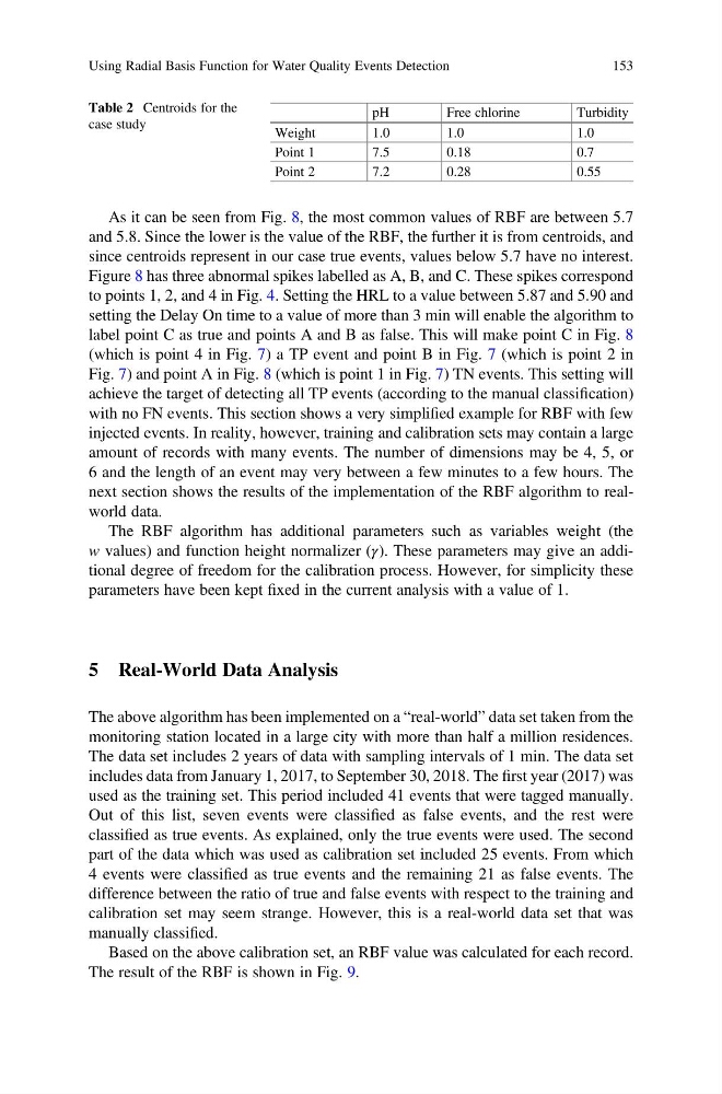
Table 2 Centroids for the
case study
pH
Free chlorine
Turbidity
Weight
1.0
1.0
1.0
Point 1
7.5
0.18
0.7
Point 2
7.2
0.28
0.55
Using Radial Basis Function for Water Quality Events Detection
153
and 5.8. Since the lower is the value of the RBF, the further it is from centroids, and
since centroids represent in our case true events, values below 5.7 have no interest.
Figure 8 has three abnormal spikes labelled as A, B, and C. These spikes correspond
to points 1, 2, and 4 in Fig. 4. Setting the HRL to a value between 5.87 and 5.90 and
setting the Delay On time to a value of more than 3 min will enable the algorithm to
label point C as true and points A and B as false. This will make point C in Fig. 8
(which is point 4 in Fig. 7) a TP event and point B in Fig. 7 (which is point 2 in
Fig. 7) and point A in Fig. 8 (which is point 1 in Fig. 7) TN events. This setting will
achieve the target of detecting all TP events (according to the manual classification)
with no FN events. This section shows a very simplified example for RBF with few
injected events. In reality, however, training and calibration sets may contain a large
amount of records with many events. The number of dimensions may be 4, 5, or
6 and the length of an event may very between a few minutes to a few hours. The
next section shows the results of the implementation of the RBF algorithm to realworld data.
The RBF algorithm has additional parameters such as variables weight (the
w values) and function height normalizer (γ). These parameters may give an additional degree of freedom for the calibration process. However, for simplicity these
parameters have been kept fixed in the current analysis with a value of 1.
5 Real-World Data Analysis
The above algorithm has been implemented on a “real-world” data set taken from the
monitoring station located in a large city with more than half a million residences.
The data set includes 2 years of data with sampling intervals of 1 min. The data set
includes data from January 1, 2017, to September 30, 2018. The first year (2017) was
used as the training set. This period included 41 events that were tagged manually.
Out of this list, seven events were classified as false events, and the rest were
classified as true events. As explained, only the true events were used. The second
part of the data which was used as calibration set included 25 events. From which
4 events were classified as true events and the remaining 21 as false events. The
difference between the ratio of true and false events with respect to the training and
calibration set may seem strange. However, this is a real-world data set that was
manually classified.
Based on the above calibration set, an RBF value was calculated for each record.
The result of the RBF is shown in Fig. 9.
Table 2 Centroids for the
case study
pH
Free chlorine
Turbidity
Weight
1.0
1.0
1.0
Point 1
7.5
0.18
0.7
Point 2
7.2
0.28
0.55
Using Radial Basis Function for Water Quality Events Detection
153