

4 An Illustrative Case Study
This section describes a numerical example, which implements the above framework, and utilizes laboratory rig generated results. The purpose of this example is to
demonstrate the implementation of the algorithm to a level in which the reader can
follow the calculation results. The data set in this example contains 1-day samples
with several artificial events than have been injected into the data in order to illustrate
the detection of these events using the RBF.
Figure 7 shows a 1-day chart of water quality with three measurements: turbidity,
free chlorine, and pH.
Data is recorded with 5-min intervals between records. This gives 24Ã12 ¼ 288
records per day. The pH measurement is displayed with blue color. Its actual range
varies between 7.0 and 7.5 with two local peaks at a level near 8.0 around record
190 and 270. The free chlorine and turbidity are displayed with green and red colors,
respectively. Turbidity normal level is around 0.37, and free chlorine normal level
oscillates around 0.4 with two additional noise effects. First, during midday (around
record number 140) when the temperature is high, the level of free chlorine is lower
due to extensive evaporation. Second, the level of free chlorine is affected by the
dosing system which works in “open loop control.” These two effects create the
smooth U shape with hourly fluctuation of the free chlorine curve.
Five abnormal events can be noticed in Fig. 7. They are numbered 1–5. Events
1, 2, 3, and 5 were classified as false. Only event 4 was classified as true by an expert.
The task now is to calibrate parameter values of the RBF algorithm in order to
achieve the same classification. The steps for the manual calculation to obtain the
optimal values are explained below.
The five events shown in Fig. 7 form the calibration set. The training set for this
problem includes two points. These points are listed in Table 2.
Given the values of the centroids in Table 2 for each point in Fig. 7, a value of
RBF was calculated based on the inner part of Eq. 2. For example, the value for the
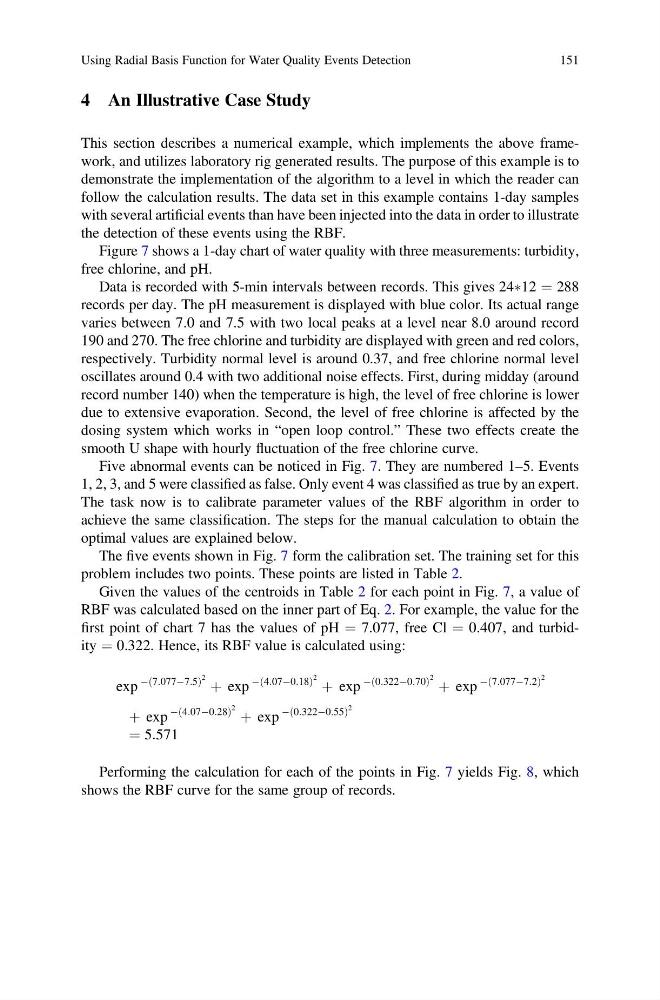
first point of chart 7 has the values of pH ¼ 7.077, free Cl ¼ 0.407, and turbidity ¼ 0.322. Hence, its RBF value is calculated using:
exp
À 7:077À7:5
ð
Þ
2 þ exp
À 4:07À0:18
ð
Þ
2 þ exp
À 0:322À0:70
ð
Þ
2 þ exp
À 7:077À7:2
ð
Þ
2
þ exp
À 4:07À0:28
ð
Þ
2 þ exp
À 0:322À0:55
ð
Þ
2
¼ 5:571
Performing the calculation for each of the points in Fig. 7 yields Fig. 8, which
shows the RBF curve for the same group of records.
Using Radial Basis Function for Water Quality Events Detection
151
This section describes a numerical example, which implements the above framework, and utilizes laboratory rig generated results. The purpose of this example is to
demonstrate the implementation of the algorithm to a level in which the reader can
follow the calculation results. The data set in this example contains 1-day samples
with several artificial events than have been injected into the data in order to illustrate
the detection of these events using the RBF.
Figure 7 shows a 1-day chart of water quality with three measurements: turbidity,
free chlorine, and pH.
Data is recorded with 5-min intervals between records. This gives 24Ã12 ¼ 288
records per day. The pH measurement is displayed with blue color. Its actual range
varies between 7.0 and 7.5 with two local peaks at a level near 8.0 around record
190 and 270. The free chlorine and turbidity are displayed with green and red colors,
respectively. Turbidity normal level is around 0.37, and free chlorine normal level
oscillates around 0.4 with two additional noise effects. First, during midday (around
record number 140) when the temperature is high, the level of free chlorine is lower
due to extensive evaporation. Second, the level of free chlorine is affected by the
dosing system which works in “open loop control.” These two effects create the
smooth U shape with hourly fluctuation of the free chlorine curve.
Five abnormal events can be noticed in Fig. 7. They are numbered 1–5. Events
1, 2, 3, and 5 were classified as false. Only event 4 was classified as true by an expert.
The task now is to calibrate parameter values of the RBF algorithm in order to
achieve the same classification. The steps for the manual calculation to obtain the
optimal values are explained below.
The five events shown in Fig. 7 form the calibration set. The training set for this
problem includes two points. These points are listed in Table 2.
Given the values of the centroids in Table 2 for each point in Fig. 7, a value of
RBF was calculated based on the inner part of Eq. 2. For example, the value for the
first point of chart 7 has the values of pH ¼ 7.077, free Cl ¼ 0.407, and turbidity ¼ 0.322. Hence, its RBF value is calculated using:
exp
À 7:077À7:5
ð
Þ
2 þ exp
À 4:07À0:18
ð
Þ
2 þ exp
À 0:322À0:70
ð
Þ
2 þ exp
À 7:077À7:2
ð
Þ
2
þ exp
À 4:07À0:28
ð
Þ
2 þ exp
À 0:322À0:55
ð
Þ
2
¼ 5:571
Performing the calculation for each of the points in Fig. 7 yields Fig. 8, which
shows the RBF curve for the same group of records.
Using Radial Basis Function for Water Quality Events Detection
151