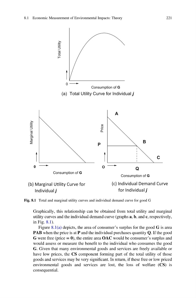
Graphically, this relationship can be obtained from total utility and marginal
utility curves and the individual demand curve (graphs a, b, and c, respectively,
in Fig. 8.1).
Figure 8.1(a) depicts, the area of consumer’s surplus for the good G is area
PAB when the price is at P and the individual purchases quantity Q. If the good
G were free (price = 0), the entire area OAC would be consumer’s surplus and
would assess or measure the benefit to the individual who consumes the good
G. Given that many environmental goods and services are freely available or
have low prices, the CS component forming part of the total utility of those
goods and services may be very significant. In return, if these free or low priced
environmental goods and services are lost, the loss of welfare (CS) is
consequential.
(a) Total Utility Curve for Individual j
(b) Marginal UƟlity Curve for
Individual j
(c) Individual Demand Curve
for Individual j
Consumption of G
Consumption of G
Consumption of G
Price
Marginal Utility
O
0
0
B
A
P
C
Q
Total Utility
Fig. 8.1 Total and marginal utility curves and individual demand curve for good G
8.1 Economic Measurement of Environmental Impacts: Theory
221