

In semiconductor and the fiber-optical lasers, the geometric length of the resonator is much more than the wavelength of the generated optical emission, and the
oscillation frequency is close to the natural frequency of the optical resonator. We
use the semiclassical representation of Maxwell equation for the double-level system
in the dipole approximation.
For small perturbations, in Chap. 3, the system of three equations was investigated for the strength of the electromagnetic field E n (t) ¼ E L (t), for the polarization
P n (t) of the QWLD active material and the population difference N(t) between
excited and non-excited levels of the laser active element. Taking into consideration
the transformations made in Chap. 3, the system of differential equations (Eq. 5.35)
for the single-frequency single-type mode, when the only main type of spatial
oscillations is excited in the resonator, is added by the Langevinian noise sources
ξ E , ξ P , ξ N , which takes into account, relatively, the amplitude noise of the QWLD
emission, the medium polarization noise, and the spontaneous noise of the active
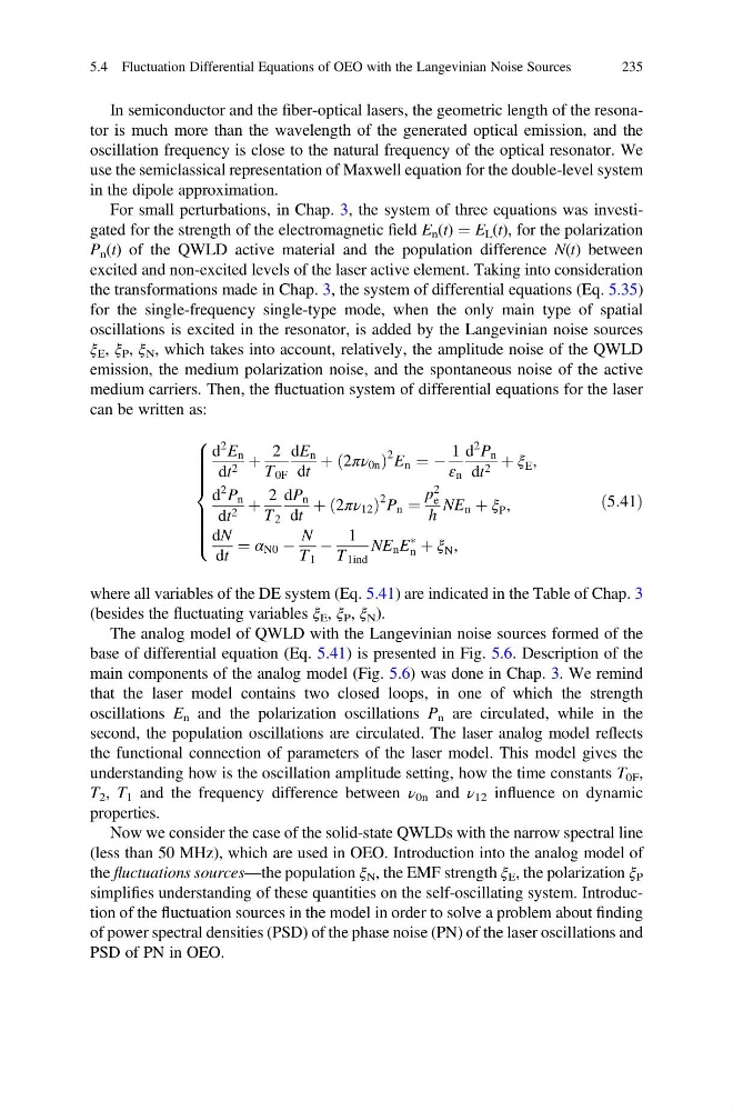
medium carriers. Then, the fluctuation system of differential equations for the laser
can be written as:
d
2 E n
dt 2 þ
2
T 0F
dE n
dt
þ 2πν 0n
ð
Þ
2 E n ¼ À
1
ε n
d
2 P n
dt 2 þ ξ E ,
d
2 P n
dt 2 þ
2
T 2
dP n
dt
þ 2πν 12
ð
Þ
2 P n ¼
p
2
e
h
NE n þ ξ P ,
dN
dt
¼ α N0 À
N
T 1
À
1
T 1ind
NE n E
Ã
n þ ξ N ,
8
> > > > > > <
> > > > > > :
ð5:41Þ
where all variables of the DE system (Eq. 5.41) are indicated in the Table of Chap. 3
(besides the fluctuating variables ξ E , ξ P , ξ N ).
The analog model of QWLD with the Langevinian noise sources formed of the
base of differential equation (Eq. 5.41) is presented in Fig. 5.6. Description of the
main components of the analog model (Fig. 5.6) was done in Chap. 3. We remind
that the laser model contains two closed loops, in one of which the strength
oscillations E n and the polarization oscillations P n are circulated, while in the
second, the population oscillations are circulated. The laser analog model reflects
the functional connection of parameters of the laser model. This model gives the
understanding how is the oscillation amplitude setting, how the time constants T 0F ,
T 2 , T 1 and the frequency difference between ν 0n and ν 12 influence on dynamic
properties.
Now we consider the case of the solid-state QWLDs with the narrow spectral line
(less than 50 MHz), which are used in OEO. Introduction into the analog model of
the fluctuations sources—the population ξ N , the EMF strength ξ E , the polarization ξ P
simplifies understanding of these quantities on the self-oscillating system. Introduction of the fluctuation sources in the model in order to solve a problem about finding
of power spectral densities (PSD) of the phase noise (PN) of the laser oscillations and
PSD of PN in OEO.
5.4 Fluctuation Differential Equations of OEO with the Langevinian Noise Sources
235
oscillation frequency is close to the natural frequency of the optical resonator. We
use the semiclassical representation of Maxwell equation for the double-level system
in the dipole approximation.
For small perturbations, in Chap. 3, the system of three equations was investigated for the strength of the electromagnetic field E n (t) ¼ E L (t), for the polarization
P n (t) of the QWLD active material and the population difference N(t) between
excited and non-excited levels of the laser active element. Taking into consideration
the transformations made in Chap. 3, the system of differential equations (Eq. 5.35)
for the single-frequency single-type mode, when the only main type of spatial
oscillations is excited in the resonator, is added by the Langevinian noise sources
ξ E , ξ P , ξ N , which takes into account, relatively, the amplitude noise of the QWLD
emission, the medium polarization noise, and the spontaneous noise of the active
medium carriers. Then, the fluctuation system of differential equations for the laser
can be written as:
d
2 E n
dt 2 þ
2
T 0F
dE n
dt
þ 2πν 0n
ð
Þ
2 E n ¼ À
1
ε n
d
2 P n
dt 2 þ ξ E ,
d
2 P n
dt 2 þ
2
T 2
dP n
dt
þ 2πν 12
ð
Þ
2 P n ¼
p
2
e
h
NE n þ ξ P ,
dN
dt
¼ α N0 À
N
T 1
À
1
T 1ind
NE n E
Ã
n þ ξ N ,
8
> > > > > > <
> > > > > > :
ð5:41Þ
where all variables of the DE system (Eq. 5.41) are indicated in the Table of Chap. 3
(besides the fluctuating variables ξ E , ξ P , ξ N ).
The analog model of QWLD with the Langevinian noise sources formed of the
base of differential equation (Eq. 5.41) is presented in Fig. 5.6. Description of the
main components of the analog model (Fig. 5.6) was done in Chap. 3. We remind
that the laser model contains two closed loops, in one of which the strength
oscillations E n and the polarization oscillations P n are circulated, while in the
second, the population oscillations are circulated. The laser analog model reflects
the functional connection of parameters of the laser model. This model gives the
understanding how is the oscillation amplitude setting, how the time constants T 0F ,
T 2 , T 1 and the frequency difference between ν 0n and ν 12 influence on dynamic
properties.
Now we consider the case of the solid-state QWLDs with the narrow spectral line
(less than 50 MHz), which are used in OEO. Introduction into the analog model of
the fluctuations sources—the population ξ N , the EMF strength ξ E , the polarization ξ P
simplifies understanding of these quantities on the self-oscillating system. Introduction of the fluctuation sources in the model in order to solve a problem about finding
of power spectral densities (PSD) of the phase noise (PN) of the laser oscillations and
PSD of PN in OEO.
5.4 Fluctuation Differential Equations of OEO with the Langevinian Noise Sources
235