

pE
2
0L ¼ G 0 E
2
0L N 0L À E
2
0L =T 0F ,
pN 0L ¼ α N0 J 0N þ J 10
ð
ÞÀ 1=T 1
ð
ÞN À G 00 N 0L E
2
0L ,
p
2
þ
1
T F
p þ 2π f eF0 Æ ν 0F
ð
Þ
2
!
U ¼ pS NY E
2
0L K MZ K FOS K PD U
Â
Ã
:
8
> > > <
> > > :
,
ð5:21Þ
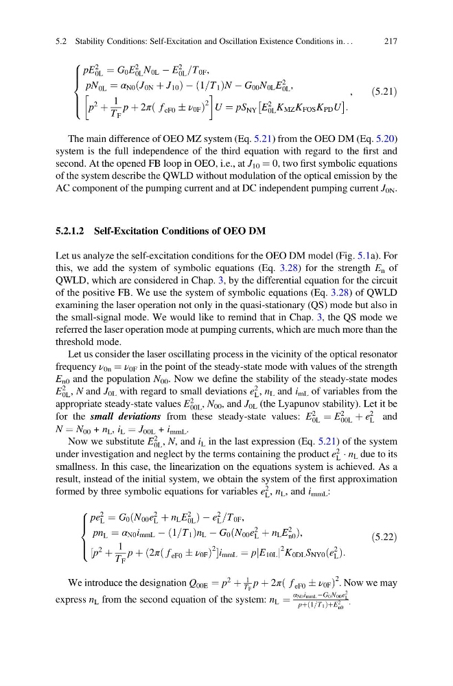
The main difference of OEO MZ system (Eq. 5.21) from the OEO DM (Eq. 5.20)
system is the full independence of the third equation with regard to the first and
second. At the opened FB loop in OEO, i.e., at J 10 ¼ 0, two first symbolic equations
of the system describe the QWLD without modulation of the optical emission by the
AC component of the pumping current and at DC independent pumping current J 0N .
5.2.1.2 Self-Excitation Conditions of OEO DM
Let us analyze the self-excitation conditions for the OEO DM model (Fig. 5.1a). For
this, we add the system of symbolic equations (Eq. 3.28) for the strength E n of
QWLD, which are considered in Chap. 3, by the differential equation for the circuit
of the positive FB. We use the system of symbolic equations (Eq. 3.28) of QWLD
examining the laser operation not only in the quasi-stationary (QS) mode but also in
the small-signal mode. We would like to remind that in Chap. 3, the QS mode we
referred the laser operation mode at pumping currents, which are much more than the
threshold mode.
Let us consider the laser oscillating process in the vicinity of the optical resonator
frequency ν 0n ¼ ν 0F in the point of the steady-state mode with values of the strength
E n0 and the population N 00 . Now we define the stability of the steady-state modes
E
2
0L , N and J 0L with regard to small deviations e
2
L , n L and i mL of variables from the
appropriate steady-state values E
2
00L , N 00 , and J 0L (the Lyapunov stability). Let it be
for the small deviations from these steady-state values: E
2
0L ¼ E
2
00L þ e
2
L and
N ¼ N 00 + n L , i L ¼ J 00L + i mmL .
Now we substitute E
2
0L , N, and i L in the last expression (Eq. 5.21) of the system
under investigation and neglect by the terms containing the product e
2
L Á n L due to its
smallness. In this case, the linearization on the equations system is achieved. As a
result, instead of the initial system, we obtain the system of the first approximation
formed by three symbolic equations for variables e
2
L , n L , and i mmL :
pe
2
L ¼ G 0 ðN 00 e
2
L þ n L E
2
0L Þ À e
2
L =T 0F ,
pn L ¼ α N0 i mmL À ð1=T 1 Þn L À G 0 ðN 00 e
2
L þ n L E
2
n0 Þ,
½p
2
þ
1
T F
p þ ð2πð f eF0 Æ ν 0F Þ
2 i mmL ¼ pjE 10L j
2 K 0DL S NY0 ðe
2
L Þ:
8
> > <
> > :
ð5:22Þ
We introduce the designation Q 00E ¼ p
2
þ
1
T F
p þ 2π f eF0 Æ ν 0F
ð
Þ
2
. Now we may
express n L from the second equation of the system: n L ¼
α N0 i mmL ÀG 0 N 00 e
2
L
pþ 1=T 1
ð
ÞþE
2
n0
.
5.2 Stability Conditions: Self-Excitation and Oscillation Existence Conditions in. . .
217
2
0L ¼ G 0 E
2
0L N 0L À E
2
0L =T 0F ,
pN 0L ¼ α N0 J 0N þ J 10
ð
ÞÀ 1=T 1
ð
ÞN À G 00 N 0L E
2
0L ,
p
2
þ
1
T F
p þ 2π f eF0 Æ ν 0F
ð
Þ
2
!
U ¼ pS NY E
2
0L K MZ K FOS K PD U
Â
Ã
:
8
> > > <
> > > :
,
ð5:21Þ
The main difference of OEO MZ system (Eq. 5.21) from the OEO DM (Eq. 5.20)
system is the full independence of the third equation with regard to the first and
second. At the opened FB loop in OEO, i.e., at J 10 ¼ 0, two first symbolic equations
of the system describe the QWLD without modulation of the optical emission by the
AC component of the pumping current and at DC independent pumping current J 0N .
5.2.1.2 Self-Excitation Conditions of OEO DM
Let us analyze the self-excitation conditions for the OEO DM model (Fig. 5.1a). For
this, we add the system of symbolic equations (Eq. 3.28) for the strength E n of
QWLD, which are considered in Chap. 3, by the differential equation for the circuit
of the positive FB. We use the system of symbolic equations (Eq. 3.28) of QWLD
examining the laser operation not only in the quasi-stationary (QS) mode but also in
the small-signal mode. We would like to remind that in Chap. 3, the QS mode we
referred the laser operation mode at pumping currents, which are much more than the
threshold mode.
Let us consider the laser oscillating process in the vicinity of the optical resonator
frequency ν 0n ¼ ν 0F in the point of the steady-state mode with values of the strength
E n0 and the population N 00 . Now we define the stability of the steady-state modes
E
2
0L , N and J 0L with regard to small deviations e
2
L , n L and i mL of variables from the
appropriate steady-state values E
2
00L , N 00 , and J 0L (the Lyapunov stability). Let it be
for the small deviations from these steady-state values: E
2
0L ¼ E
2
00L þ e
2
L and
N ¼ N 00 + n L , i L ¼ J 00L + i mmL .
Now we substitute E
2
0L , N, and i L in the last expression (Eq. 5.21) of the system
under investigation and neglect by the terms containing the product e
2
L Á n L due to its
smallness. In this case, the linearization on the equations system is achieved. As a
result, instead of the initial system, we obtain the system of the first approximation
formed by three symbolic equations for variables e
2
L , n L , and i mmL :
pe
2
L ¼ G 0 ðN 00 e
2
L þ n L E
2
0L Þ À e
2
L =T 0F ,
pn L ¼ α N0 i mmL À ð1=T 1 Þn L À G 0 ðN 00 e
2
L þ n L E
2
n0 Þ,
½p
2
þ
1
T F
p þ ð2πð f eF0 Æ ν 0F Þ
2 i mmL ¼ pjE 10L j
2 K 0DL S NY0 ðe
2
L Þ:
8
> > <
> > :
ð5:22Þ
We introduce the designation Q 00E ¼ p
2
þ
1
T F
p þ 2π f eF0 Æ ν 0F
ð
Þ
2
. Now we may
express n L from the second equation of the system: n L ¼
α N0 i mmL ÀG 0 N 00 e
2
L
pþ 1=T 1
ð
ÞþE
2
n0
.
5.2 Stability Conditions: Self-Excitation and Oscillation Existence Conditions in. . .
217