

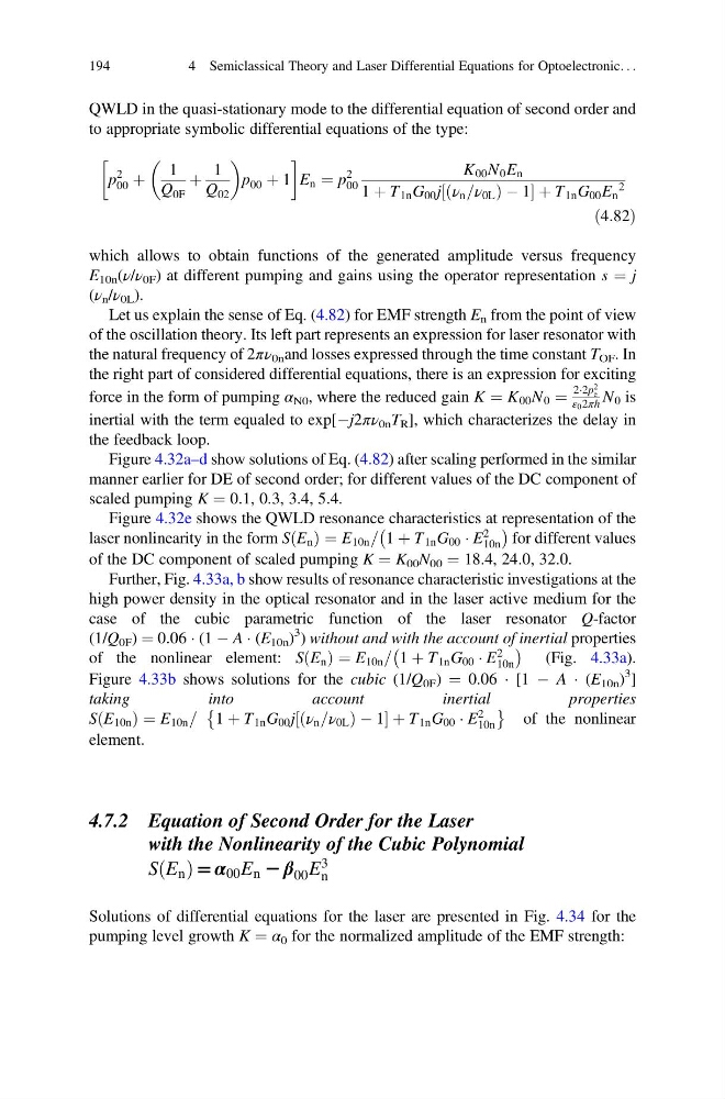
QWLD in the quasi-stationary mode to the differential equation of second order and
to appropriate symbolic differential equations of the type:
p
2
00 þ
1
Q 0F
þ
1
Q 02
p 00 þ 1
!
E n ¼ p
2
00
K 00 N 0 E n
1 þ T 1n G 00 j ν n =ν 0L
ð
ÞÀ1
½
þT 1n G 00 E n
2
ð4:82Þ
which allows to obtain functions of the generated amplitude versus frequency
E 10n (ν/ν 0F ) at different pumping and gains using the operator representation s ¼ j
(ν n /ν 0L ).
Let us explain the sense of Eq. (4.82) for EMF strength E n from the point of view
of the oscillation theory. Its left part represents an expression for laser resonator with
the natural frequency of 2πν 0n and losses expressed through the time constant T OF . In
the right part of considered differential equations, there is an expression for exciting
force in the form of pumping α N0 , where the reduced gain K ¼ K 00 N 0 ¼
2Á2p
2
e
ε 0 2πh N 0 is
inertial with the term equaled to exp[Àj2πν 0n T R ], which characterizes the delay in
the feedback loop.
Figure 4.32a–d show solutions of Eq. (4.82) after scaling performed in the similar
manner earlier for DE of second order; for different values of the DC component of
scaled pumping K ¼ 0.1, 0.3, 3.4, 5.4.
Figure 4.32e shows the QWLD resonance characteristics at representation of the
laser nonlinearity in the form S E n
ð Þ ¼ E 10n = 1 þ T 1n G 00 Á E
2
10n
À
Á
for different values
of the DC component of scaled pumping K ¼ K 00 N 00 ¼ 18.4, 24.0, 32.0.
Further, Fig. 4.33a, b show results of resonance characteristic investigations at the
high power density in the optical resonator and in the laser active medium for the
case of the cubic parametric function of the laser resonator Q-factor
(1/Q 0F ) ¼ 0.06 Á (1 À A Á (E 10n )
3 ) without and with the account of inertial properties
of the nonlinear element: S E n
ð Þ ¼ E 10n = 1 þ T 1n G 00 Á E
2
10n
À
Á
(Fig. 4.33a).
Figure 4.33b shows solutions for the cubic (1/Q 0F ) ¼ 0.06 Á [1 À A Á (E 10n )
3 ]
taking
into
account
inertial
properties
S E 10n
ð
Þ ¼ E 10n = 1 þ T 1n G 00 j ν n =ν 0L
ð
ÞÀ1
½
þT 1n G 00 Á E
2
10n
È
É
of the nonlinear
element.
4.7.2 Equation of Second Order for the Laser
with the Nonlinearity of the Cubic Polynomial
S E n
ð Þ= α 00 E n 2 β 00 E
3
n
Solutions of differential equations for the laser are presented in Fig. 4.34 for the
pumping level growth K ¼ α 0 for the normalized amplitude of the EMF strength:
194
4 Semiclassical Theory and Laser Differential Equations for Optoelectronic. . .
to appropriate symbolic differential equations of the type:
p
2
00 þ
1
Q 0F
þ
1
Q 02
p 00 þ 1
!
E n ¼ p
2
00
K 00 N 0 E n
1 þ T 1n G 00 j ν n =ν 0L
ð
ÞÀ1
½
þT 1n G 00 E n
2
ð4:82Þ
which allows to obtain functions of the generated amplitude versus frequency
E 10n (ν/ν 0F ) at different pumping and gains using the operator representation s ¼ j
(ν n /ν 0L ).
Let us explain the sense of Eq. (4.82) for EMF strength E n from the point of view
of the oscillation theory. Its left part represents an expression for laser resonator with
the natural frequency of 2πν 0n and losses expressed through the time constant T OF . In
the right part of considered differential equations, there is an expression for exciting
force in the form of pumping α N0 , where the reduced gain K ¼ K 00 N 0 ¼
2Á2p
2
e
ε 0 2πh N 0 is
inertial with the term equaled to exp[Àj2πν 0n T R ], which characterizes the delay in
the feedback loop.
Figure 4.32a–d show solutions of Eq. (4.82) after scaling performed in the similar
manner earlier for DE of second order; for different values of the DC component of
scaled pumping K ¼ 0.1, 0.3, 3.4, 5.4.
Figure 4.32e shows the QWLD resonance characteristics at representation of the
laser nonlinearity in the form S E n
ð Þ ¼ E 10n = 1 þ T 1n G 00 Á E
2
10n
À
Á
for different values
of the DC component of scaled pumping K ¼ K 00 N 00 ¼ 18.4, 24.0, 32.0.
Further, Fig. 4.33a, b show results of resonance characteristic investigations at the
high power density in the optical resonator and in the laser active medium for the
case of the cubic parametric function of the laser resonator Q-factor
(1/Q 0F ) ¼ 0.06 Á (1 À A Á (E 10n )
3 ) without and with the account of inertial properties
of the nonlinear element: S E n
ð Þ ¼ E 10n = 1 þ T 1n G 00 Á E
2
10n
À
Á
(Fig. 4.33a).
Figure 4.33b shows solutions for the cubic (1/Q 0F ) ¼ 0.06 Á [1 À A Á (E 10n )
3 ]
taking
into
account
inertial
properties
S E 10n
ð
Þ ¼ E 10n = 1 þ T 1n G 00 j ν n =ν 0L
ð
ÞÀ1
½
þT 1n G 00 Á E
2
10n
È
É
of the nonlinear
element.
4.7.2 Equation of Second Order for the Laser
with the Nonlinearity of the Cubic Polynomial
S E n
ð Þ= α 00 E n 2 β 00 E
3
n
Solutions of differential equations for the laser are presented in Fig. 4.34 for the
pumping level growth K ¼ α 0 for the normalized amplitude of the EMF strength:
194
4 Semiclassical Theory and Laser Differential Equations for Optoelectronic. . .