

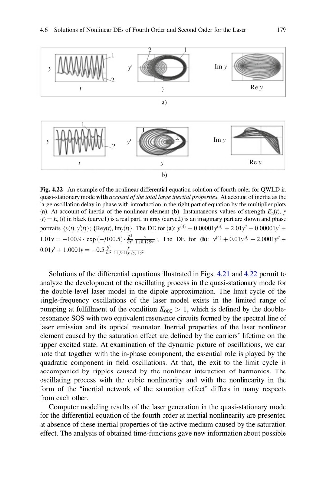
Solutions of the differential equations illustrated in Figs. 4.21 and 4.22 permit to
analyze the development of the oscillating process in the quasi-stationary mode for
the double-level laser model in the dipole approximation. The limit cycle of the
single-frequency oscillations of the laser model exists in the limited range of
pumping at fulfillment of the condition K 000 > 1, which is defined by the doubleresonance SOS with two equivalent resonance circuits formed by the spectral line of
laser emission and its optical resonator. Inertial properties of the laser nonlinear
element caused by the saturation effect are defined by the carriers’ lifetime on the
upper excited state. At examination of the dynamic picture of oscillations, we can
note that together with the in-phase component, the essential role is played by the
quadratic component in field oscillations. At that, the exit to the limit cycle is
accompanied by ripples caused by the nonlinear interaction of harmonics. The
oscillating process with the cubic nonlinearity and with the nonlinearity in the
form of the “inertial network of the saturation effect” differs in many respects
from each other.
Computer modeling results of the laser generation in the quasi-stationary mode
for the differential equation of the fourth order at inertial nonlinearity are presented
at absence of these inertial properties of the active medium caused by the saturation
effect. The analysis of obtained time-functions gave new information about possible
y
y
y’
1
2
a)
b)
2
1
Im y
Re y
t
y
y
y’
1
2
2
1
Im y
Re y
t
Fig. 4.22 An example of the nonlinear differential equation solution of fourth order for QWLD in
quasi-stationary mode with account of the total large inertial properties. At account of inertia as the
large oscillation delay in phase with introduction in the right part of equation by the multiplier plots
(a). At account of inertia of the nonlinear element (b). Instantaneous values of strength E n (t), y
(t) ¼ E n (t) in black (curve1) is a real part, in gray (curve2) is an imaginary part are shown and phase
portraits {y(t), y
0
(t)}; {Rey(t), Imy(t)}. The DE for (a): y
4
ð Þ þ 0:00001y
3
ð Þ þ 2:01y
00 þ 0:00001y
0 þ
1:01y ¼ À100:9 Á exp Àj100:5
ð
ÞÁ
∂
2
∂t 2
y
1þ0:125y 2 ; The DE for (b): y
4
ð Þ þ 0:01y
3
ð Þ þ 2:0001y
00 þ
0:01y
0 þ 1:0001y ¼ À0:5
∂
2
∂t 2
y
1þj0:1 y 0 =y
ð
Þþy 2
4.6 Solutions of Nonlinear DEs of Fourth Order and Second Order for the Laser
179
analyze the development of the oscillating process in the quasi-stationary mode for
the double-level laser model in the dipole approximation. The limit cycle of the
single-frequency oscillations of the laser model exists in the limited range of
pumping at fulfillment of the condition K 000 > 1, which is defined by the doubleresonance SOS with two equivalent resonance circuits formed by the spectral line of
laser emission and its optical resonator. Inertial properties of the laser nonlinear
element caused by the saturation effect are defined by the carriers’ lifetime on the
upper excited state. At examination of the dynamic picture of oscillations, we can
note that together with the in-phase component, the essential role is played by the
quadratic component in field oscillations. At that, the exit to the limit cycle is
accompanied by ripples caused by the nonlinear interaction of harmonics. The
oscillating process with the cubic nonlinearity and with the nonlinearity in the
form of the “inertial network of the saturation effect” differs in many respects
from each other.
Computer modeling results of the laser generation in the quasi-stationary mode
for the differential equation of the fourth order at inertial nonlinearity are presented
at absence of these inertial properties of the active medium caused by the saturation
effect. The analysis of obtained time-functions gave new information about possible
y
y
y’
1
2
a)
b)
2
1
Im y
Re y
t
y
y
y’
1
2
2
1
Im y
Re y
t
Fig. 4.22 An example of the nonlinear differential equation solution of fourth order for QWLD in
quasi-stationary mode with account of the total large inertial properties. At account of inertia as the
large oscillation delay in phase with introduction in the right part of equation by the multiplier plots
(a). At account of inertia of the nonlinear element (b). Instantaneous values of strength E n (t), y
(t) ¼ E n (t) in black (curve1) is a real part, in gray (curve2) is an imaginary part are shown and phase
portraits {y(t), y
0
(t)}; {Rey(t), Imy(t)}. The DE for (a): y
4
ð Þ þ 0:00001y
3
ð Þ þ 2:01y
00 þ 0:00001y
0 þ
1:01y ¼ À100:9 Á exp Àj100:5
ð
ÞÁ
∂
2
∂t 2
y
1þ0:125y 2 ; The DE for (b): y
4
ð Þ þ 0:01y
3
ð Þ þ 2:0001y
00 þ
0:01y
0 þ 1:0001y ¼ À0:5
∂
2
∂t 2
y
1þj0:1 y 0 =y
ð
Þþy 2
4.6 Solutions of Nonlinear DEs of Fourth Order and Second Order for the Laser
179