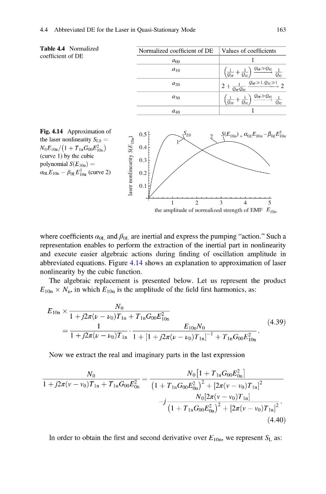
where coefficients α 0L and β 0L are inertial and express the pumping “action.” Such a
representation enables to perform the extraction of the inertial part in nonlinearity
and execute easier algebraic actions during finding of oscillation amplitude in
abbreviated equations. Figure 4.14 shows an explanation to approximation of laser
nonlinearity by the cubic function.
The algebraic replacement is presented below. Let us represent the product
E 10n  N n , in which E 10n is the amplitude of the field first harmonics, as:
E 10n Â
N 0
1 þ j2π ν À ν 0
ð
ÞT 1n þ T 1n G 00 E
2
10n
¼
1
1 þ j2π ν À ν 0
ð
ÞT 1n
Á
E 10n N 0
1 þ 1 þ j2π ν À ν 0
ð
ÞT 1n
½
Š
À1 þ T 1n G 00 E
2
10n
:
ð4:39Þ
Now we extract the real and imaginary parts in the last expression
N 0
1 þ j2π v À v 0
ð
ÞT 1n þ T 1n G 00 E
2
0n
¼
N 0 1 þ T 1n G 00 E
2
0n
Â
Ã
1 þ T 1n G 00 E
2
0n
À
Á 2 þ 2π v À v 0
ð
ÞT 1n
½
Š
2
Àj
N 0 2π v À v 0
ð
ÞT 1n
½
Š
1 þ T 1n G 00 E
2
0n
À
Á 2 þ 2π v À v 0
ð
ÞT 1n
½
Š
2
:
ð4:40Þ
In order to obtain the first and second derivative over E 10n , we represent S L as:
Table 4.4 Normalized
coefficient of DE
Normalized coefficient of DE Values of coefficients
а 00
1
a 10
1
Q 0F
þ
1
Q 02
ƒƒƒƒ!
Q 0F )Q 02 1
Q 02
a 20
2 þ
1
Q 0F Q 02
ƒƒƒƒƒƒƒ ƒ!
Q 0F )1, Q 02 )1 2
a 30
1
Q 0F
þ
1
Q 02
ƒƒƒƒ!
Q 0F )Q 02 1
Q 02
a 40
1
0.5
0.4
0.3
laser nonlinearity S(E
10n )
0.2
0.1
1
2
the amplitude of normalized strength of EMF
3
4
5
E 10n
S(E 10n ) = α 0L E 10n – β 0L E 3
10n
S L0
1
2
Fig. 4.14 Approximation of
the laser nonlinearity S L0 ¼
N 0 E 10n = 1 þ T 1n G 00 E
2
10n
À
Á
(curve 1) by the cubic
polynomial S E 10n
ð
Þ¼
α 0L E 10n À β 0L E
3
10n (curve 2)
4.4 Abbreviated DE for the Laser in Quasi-Stationary Mode
163