

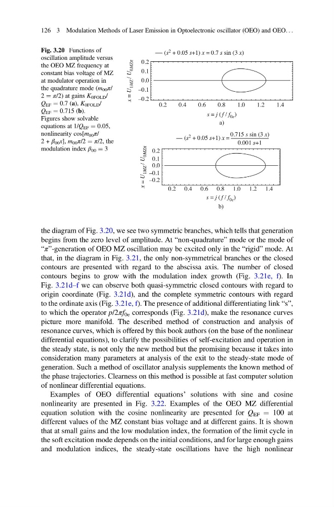
the diagram of Fig. 3.20, we see two symmetric branches, which tells that generation
begins from the zero level of amplitude. At “non-quadrature” mode or the mode of
“π”-generation of OEO MZ oscillation may be excited only in the “rigid” mode. At
that, in the diagram in Fig. 3.21, the only non-symmetrical branches or the closed
contours are presented with regard to the abscissa axis. The number of closed
contours begins to grow with the modulation index growth (Fig. 3.21e, f). In
Fig. 3.21d–f we can observe both quasi-symmetric closed contours with regard to
origin coordinate (Fig. 3.21d), and the complete symmetric contours with regard
to the ordinate axis (Fig. 3.21e, f). The presence of additional differentiating link “s”,
to which the operator p/2πf 0e corresponds (Fig. 3.21d), make the resonance curves
picture more manifold. The described method of construction and analysis of
resonance curves, which is offered by this book authors (on the base of the nonlinear
differential equations), to clarify the possibilities of self-excitation and operation in
the steady state, is not only the new method but the promising because it takes into
consideration many parameters at analysis of the exit to the steady-state mode of
generation. Such a method of oscillator analysis supplements the known method of
the phase trajectories. Clearness on this method is possible at fast computer solution
of nonlinear differential equations.
Examples of OEO differential equations’ solutions with sine and cosine
nonlinearity are presented in Fig. 3.22. Examples of the OEO MZ differential
equation solution with the cosine nonlinearity are presented for Q EF ¼ 100 at
different values of the MZ constant bias voltage and at different gains. It is shown
that at small gains and the low modulation index, the formation of the limit cycle in
the soft excitation mode depends on the initial conditions, and for large enough gains
and modulation indices, the steady-state oscillations have the high nonlinear
0.2
0.1
0.0
x
= U
1MZ / U
0MZπ
x
= U
1MZ / U
0MZπ
–0.1
–0.2
0.2
0.1
0.0
–0.1
–0.2
0.2
0.4
0.6
s = j ( f / f 0e )
0.8
a)
b)
1.0
1.2
1.4
0.2 0.4 0.6
s = j ( f / f 0e )
0.8 1.0 1.2 1.4
(s 2 + 0.05 s+1) x = 0.7 s sin (3 x)
(s 2 + 0.05 s+1) x =
0.001 s+1
0.715 s sin (3 x)
Fig. 3.20 Functions of
oscillation amplitude versus
the OEO MZ frequency at
constant bias voltage of MZ
at modulator operation in
the quadrature mode (m 00 π/
2 ¼ π/2) at gains K 0FOLD /
Q EF ¼ 0.7 (a), K 0FOLD /
Q EF ¼ 0.715 (b).
Figures show solvable
equations at 1/Q EF ¼ 0.05,
nonlinearity cos[m 00 π/
2 + β 00 x], m 00 π/2 ¼ π/2, the
modulation index β 00 ¼ 3
126 3 Modulation Methods of Laser Emission in Optoelectronic oscillator (OEO) and OEO. . .
begins from the zero level of amplitude. At “non-quadrature” mode or the mode of
“π”-generation of OEO MZ oscillation may be excited only in the “rigid” mode. At
that, in the diagram in Fig. 3.21, the only non-symmetrical branches or the closed
contours are presented with regard to the abscissa axis. The number of closed
contours begins to grow with the modulation index growth (Fig. 3.21e, f). In
Fig. 3.21d–f we can observe both quasi-symmetric closed contours with regard to
origin coordinate (Fig. 3.21d), and the complete symmetric contours with regard
to the ordinate axis (Fig. 3.21e, f). The presence of additional differentiating link “s”,
to which the operator p/2πf 0e corresponds (Fig. 3.21d), make the resonance curves
picture more manifold. The described method of construction and analysis of
resonance curves, which is offered by this book authors (on the base of the nonlinear
differential equations), to clarify the possibilities of self-excitation and operation in
the steady state, is not only the new method but the promising because it takes into
consideration many parameters at analysis of the exit to the steady-state mode of
generation. Such a method of oscillator analysis supplements the known method of
the phase trajectories. Clearness on this method is possible at fast computer solution
of nonlinear differential equations.
Examples of OEO differential equations’ solutions with sine and cosine
nonlinearity are presented in Fig. 3.22. Examples of the OEO MZ differential
equation solution with the cosine nonlinearity are presented for Q EF ¼ 100 at
different values of the MZ constant bias voltage and at different gains. It is shown
that at small gains and the low modulation index, the formation of the limit cycle in
the soft excitation mode depends on the initial conditions, and for large enough gains
and modulation indices, the steady-state oscillations have the high nonlinear
0.2
0.1
0.0
x
= U
1MZ / U
0MZπ
x
= U
1MZ / U
0MZπ
–0.1
–0.2
0.2
0.1
0.0
–0.1
–0.2
0.2
0.4
0.6
s = j ( f / f 0e )
0.8
a)
b)
1.0
1.2
1.4
0.2 0.4 0.6
s = j ( f / f 0e )
0.8 1.0 1.2 1.4
(s 2 + 0.05 s+1) x = 0.7 s sin (3 x)
(s 2 + 0.05 s+1) x =
0.001 s+1
0.715 s sin (3 x)
Fig. 3.20 Functions of
oscillation amplitude versus
the OEO MZ frequency at
constant bias voltage of MZ
at modulator operation in
the quadrature mode (m 00 π/
2 ¼ π/2) at gains K 0FOLD /
Q EF ¼ 0.7 (a), K 0FOLD /
Q EF ¼ 0.715 (b).
Figures show solvable
equations at 1/Q EF ¼ 0.05,
nonlinearity cos[m 00 π/
2 + β 00 x], m 00 π/2 ¼ π/2, the
modulation index β 00 ¼ 3
126 3 Modulation Methods of Laser Emission in Optoelectronic oscillator (OEO) and OEO. . .