

U 10MZ ¼ K 0FODL S 1A =2U 0MZπ
ð
Þ cos 2π f 0e T FOS
½
Á sin π U 0MZ À U 10MZ
ð
Þ =2U 0MZπ
½
,
sin 2π f 0e T FOS
½
¼0:
&
ð3:60Þ
The first equation of the system (Eq. 3.60), at introducing of the following
variables X ¼ πU 0MZ /2U 0MZπ , Y ¼ πU 10MZ /2U 0MZπ , K 000 ¼ K 0FODL Á (S 1A /
2U 0MZπ ) Á cos[2πf 0e T FOS ], has a form X ¼ K 000 Á sin(X À Y ), and can be solved
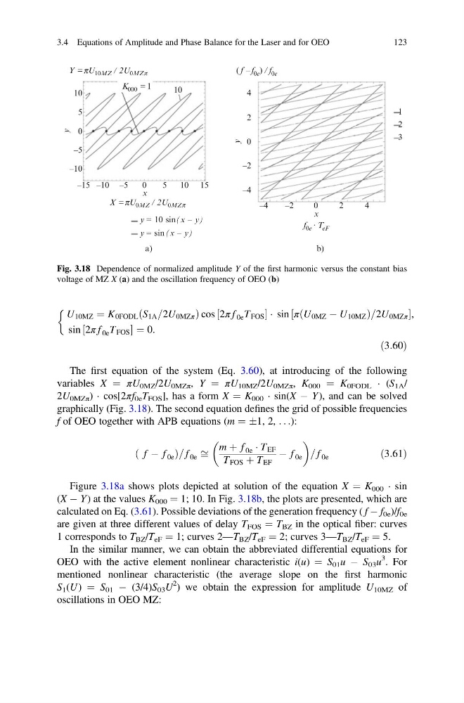
graphically (Fig. 3.18). The second equation defines the grid of possible frequencies
f of OEO together with APB equations (m ¼ Æ1, 2, . . .):
f À f 0e
ð
Þ = f 0e ffi
m þ f 0e Á T EF
T FOS þ T EF
À f 0e
= f 0e
ð3:61Þ
Figure 3.18a shows plots depicted at solution of the equation X ¼ K 000 Á sin
(X À Y ) at the values K 000 ¼ 1; 10. In Fig. 3.18b, the plots are presented, which are
calculated on Eq. (3.61). Possible deviations of the generation frequency ( f À f 0e )/f 0e
are given at three different values of delay T FOS ¼ T BZ in the optical fiber: curves
1 corresponds to T BZ /T eF ¼ 1; curves 2—T BZ /T eF ¼ 2; curves 3—T BZ /T eF ¼ 5.
In the similar manner, we can obtain the abbreviated differential equations for
OEO with the active element nonlinear characteristic i(u) ¼ S 01 u À S 03 u
3 . For
mentioned nonlinear characteristic (the average slope on the first harmonic
S 1 (U ) ¼ S 01 À (3/4)S 03 U
2 ) we obtain the expression for amplitude U 10MZ of
oscillations in OEO MZ:
10
4
1
2
3
2
0
–2
–4
–4
–2
0
2
4
10
5
0
y
y
–5
–10
–15 –10 –5
0
a)
b)
X = pU 0MZ / 2U 0MZp
pU 10MZ / 2U 0MZp
Y =
K 000 = 1
x
y = 10 sin (x – y)
y = sin (x – y)
x
f 0e · T eF
( f – f 0e ) / f 0e
5
10 15
Fig. 3.18 Dependence of normalized amplitude Y of the first harmonic versus the constant bias
voltage of MZ X (a) and the oscillation frequency of OEO (b)
3.4 Equations of Amplitude and Phase Balance for the Laser and for OEO
123
ð
Þ cos 2π f 0e T FOS
½
Á sin π U 0MZ À U 10MZ
ð
Þ =2U 0MZπ
½
,
sin 2π f 0e T FOS
½
¼0:
&
ð3:60Þ
The first equation of the system (Eq. 3.60), at introducing of the following
variables X ¼ πU 0MZ /2U 0MZπ , Y ¼ πU 10MZ /2U 0MZπ , K 000 ¼ K 0FODL Á (S 1A /
2U 0MZπ ) Á cos[2πf 0e T FOS ], has a form X ¼ K 000 Á sin(X À Y ), and can be solved
graphically (Fig. 3.18). The second equation defines the grid of possible frequencies
f of OEO together with APB equations (m ¼ Æ1, 2, . . .):
f À f 0e
ð
Þ = f 0e ffi
m þ f 0e Á T EF
T FOS þ T EF
À f 0e
= f 0e
ð3:61Þ
Figure 3.18a shows plots depicted at solution of the equation X ¼ K 000 Á sin
(X À Y ) at the values K 000 ¼ 1; 10. In Fig. 3.18b, the plots are presented, which are
calculated on Eq. (3.61). Possible deviations of the generation frequency ( f À f 0e )/f 0e
are given at three different values of delay T FOS ¼ T BZ in the optical fiber: curves
1 corresponds to T BZ /T eF ¼ 1; curves 2—T BZ /T eF ¼ 2; curves 3—T BZ /T eF ¼ 5.
In the similar manner, we can obtain the abbreviated differential equations for
OEO with the active element nonlinear characteristic i(u) ¼ S 01 u À S 03 u
3 . For
mentioned nonlinear characteristic (the average slope on the first harmonic
S 1 (U ) ¼ S 01 À (3/4)S 03 U
2 ) we obtain the expression for amplitude U 10MZ of
oscillations in OEO MZ:
10
4
1
2
3
2
0
–2
–4
–4
–2
0
2
4
10
5
0
y
y
–5
–10
–15 –10 –5
0
a)
b)
X = pU 0MZ / 2U 0MZp
pU 10MZ / 2U 0MZp
Y =
K 000 = 1
x
y = 10 sin (x – y)
y = sin (x – y)
x
f 0e · T eF
( f – f 0e ) / f 0e
5
10 15
Fig. 3.18 Dependence of normalized amplitude Y of the first harmonic versus the constant bias
voltage of MZ X (a) and the oscillation frequency of OEO (b)
3.4 Equations of Amplitude and Phase Balance for the Laser and for OEO
123