

562
13 Modeling Biological Systems
the map gives solutions which fall to zero. This should not surprise us, because
r < 1 corresponds to α < 0, which is a negative birth rate (which really becomes
part of the death rate). If 1 < r < 3, as i increases, x i approaches 1 − r −1 . If
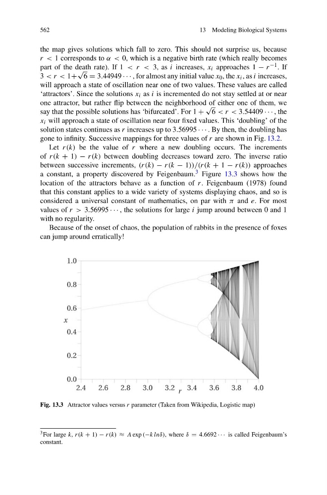
3 < r < 1+
√
6 = 3.44949 · · · , for almost any initial value x 0 , the x i , as i increases,
will approach a state of oscillation near one of two values. These values are called
‘attractors’. Since the solutions x i as i is incremented do not stay settled at or near
one attractor, but rather flip between the neighborhood of either one of them, we
say that the possible solutions has ‘bifurcated’. For 1 +
√
6 < r < 3.54409 · · · , the
x i will approach a state of oscillation near four fixed values. This ‘doubling’ of the
solution states continues as r increases up to 3.56995 · · · . By then, the doubling has
gone to infinity. Successive mappings for three values of r are shown in Fig. 13.2.
Let r(k) be the value of r where a new doubling occurs. The increments
of r(k + 1) − r(k) between doubling decreases toward zero. The inverse ratio
between successive increments, (r(k) − r(k − 1))/(r(k + 1 − r(k)) approaches
a constant, a property discovered by Feigenbaum. 3 Figure 13.3 shows how the
location of the attractors behave as a function of r. Feigenbaum (1978) found
that this constant applies to a wide variety of systems displaying chaos, and so is
considered a universal constant of mathematics, on par with π and e. For most
values of r > 3.56995 · · · , the solutions for large i jump around between 0 and 1
with no regularity.
Because of the onset of chaos, the population of rabbits in the presence of foxes
can jump around erratically!
Fig. 13.3 Attractor values versus r parameter (Taken from Wikipedia, Logistic map)
3 For large k, r(k + 1) − r(k) ≈ A exp (−k lnδ), where δ = 4.6692 · · · is called Feigenbaum’s
constant.