

9.23 Non-equilibrium Thermodynamics
411
d
dt
sdV = −
J s · dA +
˙
σ dV
(9.243)
where the first term on the right is the net flux of entropy through the surface
of the volume and the second measures the production of internal entropy due to
irreversible processes. In local form, this reads
∂s
∂t
= −∇ · J s + ˙
σ .
(9.244)
Substitution from the expression for S in Eq. (9.239) gives
˙
σ =
1
T
∂E
∂t
+
p
T
∂ρ −1
∂t
−
k
μ k
T
∂n k
∂t
+ ∇ · J s ≥ 0
(9.245)
which more generally can be put into the form (from Eq. (9.240)
˙
σ = −k B
k
y k
∂(Y k /N )
∂t
+ ∇ · J s ≥ 0 .
(9.246)
Gradients across space of the intensive thermodynamic variables such as gradients of the local temperature, the density, or the chemical potential, will cause
currents J k , such as heat flow, material flow, or chemical type flow. Expanding
J k in a Taylor series in the y k , the zeroth-order term vanishes, since there will be
no current if the gradients vanish. Assuming the quantities y k do not change too
rapidly, quadratic and higher order terms can be negligible. This means there will
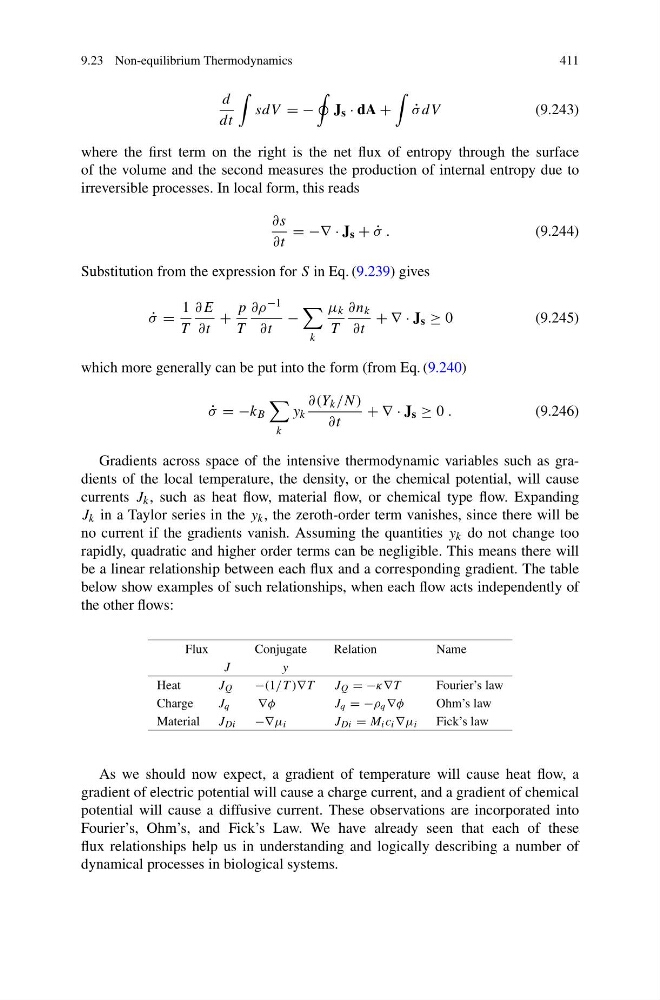
be a linear relationship between each flux and a corresponding gradient. The table
below show examples of such relationships, when each flow acts independently of
the other flows:
Flux
Conjugate
Relation
Name
J
y
Heat
J Q
−(1/T )∇T
J Q = −κ∇T
Fourier’s law
Charge
J q
∇φ
J q = −ρ q ∇φ
Ohm’s law
Material J Di
−∇μ i
J Di = M i c i ∇μ i
Fick’s law
As we should now expect, a gradient of temperature will cause heat flow, a
gradient of electric potential will cause a charge current, and a gradient of chemical
potential will cause a diffusive current. These observations are incorporated into
Fourier’s, Ohm’s, and Fick’s Law. We have already seen that each of these
flux relationships help us in understanding and logically describing a number of
dynamical processes in biological systems.
411
d
dt
sdV = −
J s · dA +
˙
σ dV
(9.243)
where the first term on the right is the net flux of entropy through the surface
of the volume and the second measures the production of internal entropy due to
irreversible processes. In local form, this reads
∂s
∂t
= −∇ · J s + ˙
σ .
(9.244)
Substitution from the expression for S in Eq. (9.239) gives
˙
σ =
1
T
∂E
∂t
+
p
T
∂ρ −1
∂t
−
k
μ k
T
∂n k
∂t
+ ∇ · J s ≥ 0
(9.245)
which more generally can be put into the form (from Eq. (9.240)
˙
σ = −k B
k
y k
∂(Y k /N )
∂t
+ ∇ · J s ≥ 0 .
(9.246)
Gradients across space of the intensive thermodynamic variables such as gradients of the local temperature, the density, or the chemical potential, will cause
currents J k , such as heat flow, material flow, or chemical type flow. Expanding
J k in a Taylor series in the y k , the zeroth-order term vanishes, since there will be
no current if the gradients vanish. Assuming the quantities y k do not change too
rapidly, quadratic and higher order terms can be negligible. This means there will
be a linear relationship between each flux and a corresponding gradient. The table
below show examples of such relationships, when each flow acts independently of
the other flows:
Flux
Conjugate
Relation
Name
J
y
Heat
J Q
−(1/T )∇T
J Q = −κ∇T
Fourier’s law
Charge
J q
∇φ
J q = −ρ q ∇φ
Ohm’s law
Material J Di
−∇μ i
J Di = M i c i ∇μ i
Fick’s law
As we should now expect, a gradient of temperature will cause heat flow, a
gradient of electric potential will cause a charge current, and a gradient of chemical
potential will cause a diffusive current. These observations are incorporated into
Fourier’s, Ohm’s, and Fick’s Law. We have already seen that each of these
flux relationships help us in understanding and logically describing a number of
dynamical processes in biological systems.