

3.2 Interactions
35
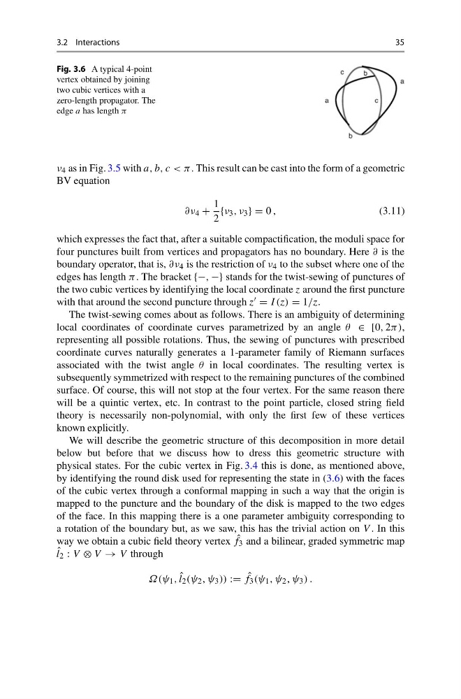
Fig. 3.6 A typical 4-point
vertex obtained by joining
two cubic vertices with a
zero-length propagator. The
edge a has length π
ν 4 as in Fig. 3.5 with a, b, c < π. This result can be cast into the form of a geometric
BV equation
∂ν 4 +
1
2
{ν 3 , ν 3 } = 0 ,
(3.11)
which expresses the fact that, after a suitable compactification, the moduli space for
four punctures built from vertices and propagators has no boundary. Here ∂ is the
boundary operator, that is, ∂ν 4 is the restriction of ν 4 to the subset where one of the
edges has length π. The bracket {−, −} stands for the twist-sewing of punctures of
the two cubic vertices by identifying the local coordinate z around the first puncture
with that around the second puncture through z = I (z) = 1/z.
The twist-sewing comes about as follows. There is an ambiguity of determining
local coordinates of coordinate curves parametrized by an angle θ ∈ [0, 2π),
representing all possible rotations. Thus, the sewing of punctures with prescribed
coordinate curves naturally generates a 1-parameter family of Riemann surfaces
associated with the twist angle θ in local coordinates. The resulting vertex is
subsequently symmetrized with respect to the remaining punctures of the combined
surface. Of course, this will not stop at the four vertex. For the same reason there
will be a quintic vertex, etc. In contrast to the point particle, closed string field
theory is necessarily non-polynomial, with only the first few of these vertices
known explicitly.
We will describe the geometric structure of this decomposition in more detail
below but before that we discuss how to dress this geometric structure with
physical states. For the cubic vertex in Fig. 3.4 this is done, as mentioned above,
by identifying the round disk used for representing the state in (3.6) with the faces
of the cubic vertex through a conformal mapping in such a way that the origin is
mapped to the puncture and the boundary of the disk is mapped to the two edges
of the face. In this mapping there is a one parameter ambiguity corresponding to
a rotation of the boundary but, as we saw, this has the trivial action on V . In this
way we obtain a cubic field theory vertex ˆ
f 3 and a bilinear, graded symmetric map
ˆ
l 2 : V ⊗ V → V through
Ω(ψ 1 , ˆ
l 2 (ψ 2 , ψ 3 )) := ˆ
f 3 (ψ 1 , ψ 2 , ψ 3 ) .
35
Fig. 3.6 A typical 4-point
vertex obtained by joining
two cubic vertices with a
zero-length propagator. The
edge a has length π
ν 4 as in Fig. 3.5 with a, b, c < π. This result can be cast into the form of a geometric
BV equation
∂ν 4 +
1
2
{ν 3 , ν 3 } = 0 ,
(3.11)
which expresses the fact that, after a suitable compactification, the moduli space for
four punctures built from vertices and propagators has no boundary. Here ∂ is the
boundary operator, that is, ∂ν 4 is the restriction of ν 4 to the subset where one of the
edges has length π. The bracket {−, −} stands for the twist-sewing of punctures of
the two cubic vertices by identifying the local coordinate z around the first puncture
with that around the second puncture through z = I (z) = 1/z.
The twist-sewing comes about as follows. There is an ambiguity of determining
local coordinates of coordinate curves parametrized by an angle θ ∈ [0, 2π),
representing all possible rotations. Thus, the sewing of punctures with prescribed
coordinate curves naturally generates a 1-parameter family of Riemann surfaces
associated with the twist angle θ in local coordinates. The resulting vertex is
subsequently symmetrized with respect to the remaining punctures of the combined
surface. Of course, this will not stop at the four vertex. For the same reason there
will be a quintic vertex, etc. In contrast to the point particle, closed string field
theory is necessarily non-polynomial, with only the first few of these vertices
known explicitly.
We will describe the geometric structure of this decomposition in more detail
below but before that we discuss how to dress this geometric structure with
physical states. For the cubic vertex in Fig. 3.4 this is done, as mentioned above,
by identifying the round disk used for representing the state in (3.6) with the faces
of the cubic vertex through a conformal mapping in such a way that the origin is
mapped to the puncture and the boundary of the disk is mapped to the two edges
of the face. In this mapping there is a one parameter ambiguity corresponding to
a rotation of the boundary but, as we saw, this has the trivial action on V . In this
way we obtain a cubic field theory vertex ˆ
f 3 and a bilinear, graded symmetric map
ˆ
l 2 : V ⊗ V → V through
Ω(ψ 1 , ˆ
l 2 (ψ 2 , ψ 3 )) := ˆ
f 3 (ψ 1 , ψ 2 , ψ 3 ) .