

6.4 Modular Operads
147
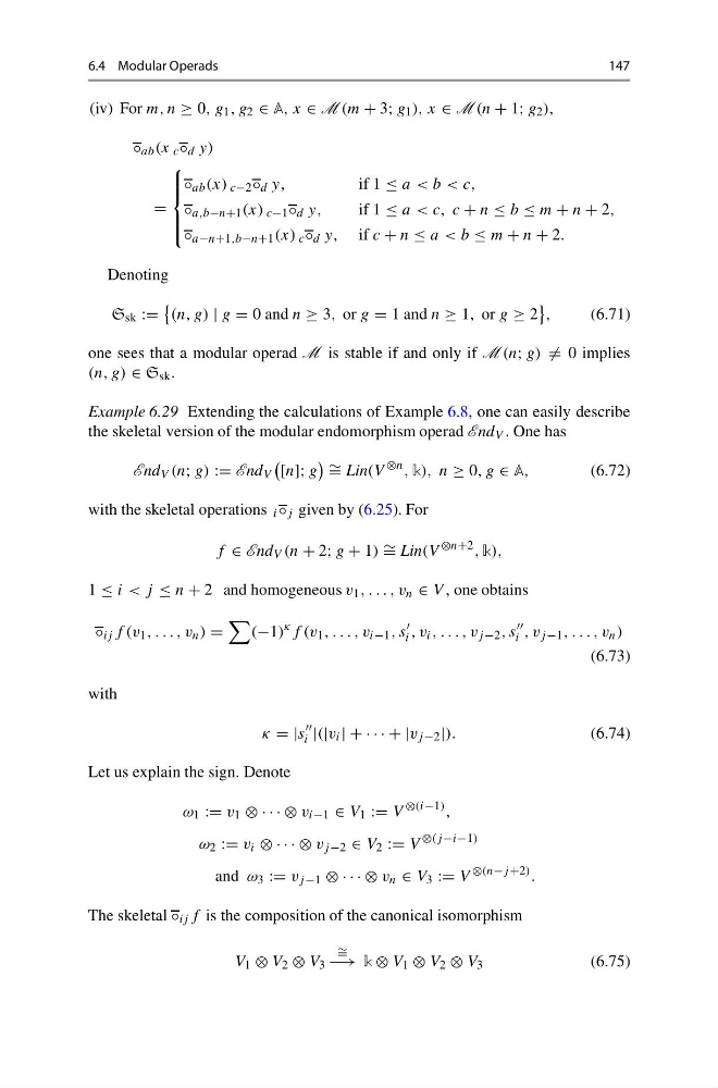
(iv) For m, n ≥ 0, g 1 , g 2 ∈ A, x ∈ M (m + 3; g 1 ), x ∈ M (n + 1; g 2 ),
◦ ab (x c ◦ d y)
=
⎧
⎪ ⎪ ⎨
⎪ ⎪ ⎩
◦ ab (x) c−2 ◦ d y,
if 1 ≤ a < b < c,
◦ a,b−n+1 (x) c−1 ◦ d y,
if 1 ≤ a < c, c + n ≤ b ≤ m + n + 2,
◦ a−n+1,b−n+1 (x) c ◦ d y, if c + n ≤ a < b ≤ m + n + 2.
Denoting
S sk :=
(n, g) | g = 0 and n ≥ 3, or g = 1 and n ≥ 1, or g ≥ 2
,
(6.71)
one sees that a modular operad M is stable if and only if M (n; g) = 0 implies
(n, g) ∈ S sk .
Example 6.29 Extending the calculations of Example 6.8, one can easily describe
the skeletal version of the modular endomorphism operad End V . One has
End V (n; g) := End V
[n]; g
∼ = Lin(V
⊗n , k), n ≥ 0, g ∈ A,
(6.72)
with the skeletal operations i ◦ j given by (6.25). For
f ∈ End V (n + 2; g + 1) ∼ = Lin(V
⊗n+2 , k),
1 ≤ i < j ≤ n + 2 and homogeneous v 1 , . . . , v n ∈ V , one obtains
◦ ij f (v 1 , . . . , v n ) =
(−1)
κ f (v 1 , . . . , v i−1 , s
i , v i , . . . , v j −2 , s
i , v j −1 , . . . , v n )
(6.73)
with
κ = |s
i |(|v i | + · · · + |v j −2 |).
(6.74)
Let us explain the sign. Denote
ω 1 := v 1 ⊗ · · · ⊗ v i−1 ∈ V 1 := V
⊗(i−1) ,
ω 2 := v i ⊗ · · · ⊗ v j −2 ∈ V 2 := V
⊗(j −i−1)
and ω 3 := v j −1 ⊗ · · · ⊗ v n ∈ V 3 := V
⊗(n−j +2) .
The skeletal ◦ ij f is the composition of the canonical isomorphism
V 1 ⊗ V 2 ⊗ V 3
∼ =
−→ k ⊗ V 1 ⊗ V 2 ⊗ V 3
(6.75)
147
(iv) For m, n ≥ 0, g 1 , g 2 ∈ A, x ∈ M (m + 3; g 1 ), x ∈ M (n + 1; g 2 ),
◦ ab (x c ◦ d y)
=
⎧
⎪ ⎪ ⎨
⎪ ⎪ ⎩
◦ ab (x) c−2 ◦ d y,
if 1 ≤ a < b < c,
◦ a,b−n+1 (x) c−1 ◦ d y,
if 1 ≤ a < c, c + n ≤ b ≤ m + n + 2,
◦ a−n+1,b−n+1 (x) c ◦ d y, if c + n ≤ a < b ≤ m + n + 2.
Denoting
S sk :=
(n, g) | g = 0 and n ≥ 3, or g = 1 and n ≥ 1, or g ≥ 2
,
(6.71)
one sees that a modular operad M is stable if and only if M (n; g) = 0 implies
(n, g) ∈ S sk .
Example 6.29 Extending the calculations of Example 6.8, one can easily describe
the skeletal version of the modular endomorphism operad End V . One has
End V (n; g) := End V
[n]; g
∼ = Lin(V
⊗n , k), n ≥ 0, g ∈ A,
(6.72)
with the skeletal operations i ◦ j given by (6.25). For
f ∈ End V (n + 2; g + 1) ∼ = Lin(V
⊗n+2 , k),
1 ≤ i < j ≤ n + 2 and homogeneous v 1 , . . . , v n ∈ V , one obtains
◦ ij f (v 1 , . . . , v n ) =
(−1)
κ f (v 1 , . . . , v i−1 , s
i , v i , . . . , v j −2 , s
i , v j −1 , . . . , v n )
(6.73)
with
κ = |s
i |(|v i | + · · · + |v j −2 |).
(6.74)
Let us explain the sign. Denote
ω 1 := v 1 ⊗ · · · ⊗ v i−1 ∈ V 1 := V
⊗(i−1) ,
ω 2 := v i ⊗ · · · ⊗ v j −2 ∈ V 2 := V
⊗(j −i−1)
and ω 3 := v j −1 ⊗ · · · ⊗ v n ∈ V 3 := V
⊗(n−j +2) .
The skeletal ◦ ij f is the composition of the canonical isomorphism
V 1 ⊗ V 2 ⊗ V 3
∼ =
−→ k ⊗ V 1 ⊗ V 2 ⊗ V 3
(6.75)