

χ
2
¼
X
i
w i y i À f h i , x
ð
Þ
½
2 þ
X
j
w j y j À f j x
ð Þ
Â
à 2
ð9Þ
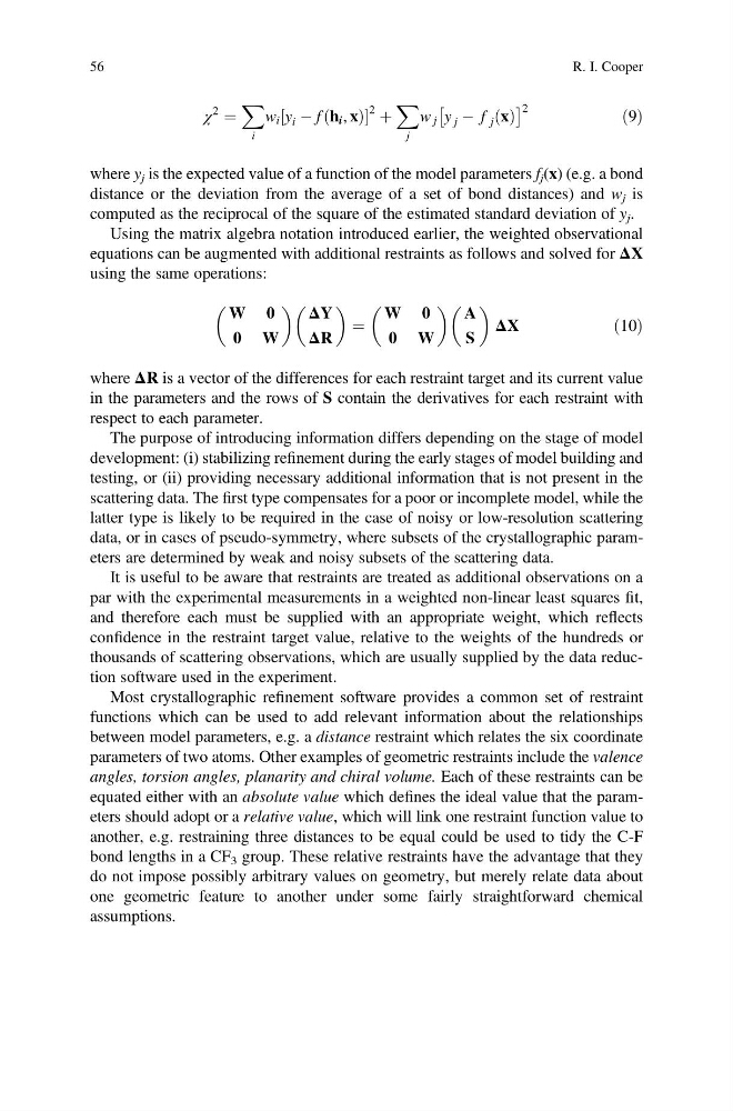
where y j is the expected value of a function of the model parameters f j (x) (e.g. a bond
distance or the deviation from the average of a set of bond distances) and w j is
computed as the reciprocal of the square of the estimated standard deviation of y j .
Using the matrix algebra notation introduced earlier, the weighted observational
equations can be augmented with additional restraints as follows and solved for ΔX
using the same operations:
W 0
0 W
ΔY
ΔR
¼
W 0
0 W
A
S
ΔX
ð10Þ
where ΔR is a vector of the differences for each restraint target and its current value
in the parameters and the rows of S contain the derivatives for each restraint with
respect to each parameter.
The purpose of introducing information differs depending on the stage of model
development: (i) stabilizing refinement during the early stages of model building and
testing, or (ii) providing necessary additional information that is not present in the
scattering data. The first type compensates for a poor or incomplete model, while the
latter type is likely to be required in the case of noisy or low-resolution scattering
data, or in cases of pseudo-symmetry, where subsets of the crystallographic parameters are determined by weak and noisy subsets of the scattering data.
It is useful to be aware that restraints are treated as additional observations on a
par with the experimental measurements in a weighted non-linear least squares fit,
and therefore each must be supplied with an appropriate weight, which reflects
confidence in the restraint target value, relative to the weights of the hundreds or
thousands of scattering observations, which are usually supplied by the data reduction software used in the experiment.
Most crystallographic refinement software provides a common set of restraint
functions which can be used to add relevant information about the relationships
between model parameters, e.g. a distance restraint which relates the six coordinate
parameters of two atoms. Other examples of geometric restraints include the valence
angles, torsion angles, planarity and chiral volume. Each of these restraints can be
equated either with an absolute value which defines the ideal value that the parameters should adopt or a relative value, which will link one restraint function value to
another, e.g. restraining three distances to be equal could be used to tidy the C-F
bond lengths in a CF 3 group. These relative restraints have the advantage that they
do not impose possibly arbitrary values on geometry, but merely relate data about
one geometric feature to another under some fairly straightforward chemical
assumptions.
56
R. I. Cooper
2
¼
X
i
w i y i À f h i , x
ð
Þ
½
2 þ
X
j
w j y j À f j x
ð Þ
Â
à 2
ð9Þ
where y j is the expected value of a function of the model parameters f j (x) (e.g. a bond
distance or the deviation from the average of a set of bond distances) and w j is
computed as the reciprocal of the square of the estimated standard deviation of y j .
Using the matrix algebra notation introduced earlier, the weighted observational
equations can be augmented with additional restraints as follows and solved for ΔX
using the same operations:
W 0
0 W
ΔY
ΔR
¼
W 0
0 W
A
S
ΔX
ð10Þ
where ΔR is a vector of the differences for each restraint target and its current value
in the parameters and the rows of S contain the derivatives for each restraint with
respect to each parameter.
The purpose of introducing information differs depending on the stage of model
development: (i) stabilizing refinement during the early stages of model building and
testing, or (ii) providing necessary additional information that is not present in the
scattering data. The first type compensates for a poor or incomplete model, while the
latter type is likely to be required in the case of noisy or low-resolution scattering
data, or in cases of pseudo-symmetry, where subsets of the crystallographic parameters are determined by weak and noisy subsets of the scattering data.
It is useful to be aware that restraints are treated as additional observations on a
par with the experimental measurements in a weighted non-linear least squares fit,
and therefore each must be supplied with an appropriate weight, which reflects
confidence in the restraint target value, relative to the weights of the hundreds or
thousands of scattering observations, which are usually supplied by the data reduction software used in the experiment.
Most crystallographic refinement software provides a common set of restraint
functions which can be used to add relevant information about the relationships
between model parameters, e.g. a distance restraint which relates the six coordinate
parameters of two atoms. Other examples of geometric restraints include the valence
angles, torsion angles, planarity and chiral volume. Each of these restraints can be
equated either with an absolute value which defines the ideal value that the parameters should adopt or a relative value, which will link one restraint function value to
another, e.g. restraining three distances to be equal could be used to tidy the C-F
bond lengths in a CF 3 group. These relative restraints have the advantage that they
do not impose possibly arbitrary values on geometry, but merely relate data about
one geometric feature to another under some fairly straightforward chemical
assumptions.
56
R. I. Cooper