

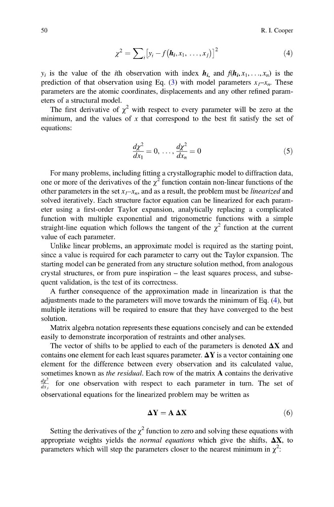
χ
2
¼
X
i
y i À f h i , x 1 , . . . , x j
À
Á
Â
à 2
ð4Þ
y i is the value of the ith observation with index h i, and f(h i , x 1 , . . ., x n ) is the
prediction of that observation using Eq. (3) with model parameters x 1 –x n . These
parameters are the atomic coordinates, displacements and any other refined parameters of a structural model.
The first derivative of χ
2 with respect to every parameter will be zero at the
minimum, and the values of x that correspond to the best fit satisfy the set of
equations:
dχ
2
dx 1
¼ 0, . . . ,
dχ
2
dx n
¼ 0
ð5Þ
For many problems, including fitting a crystallographic model to diffraction data,
one or more of the derivatives of the χ
2 function contain non-linear functions of the
other parameters in the set x 1 –x n , and as a result, the problem must be linearized and
solved iteratively. Each structure factor equation can be linearized for each parameter using a first-order Taylor expansion, analytically replacing a complicated
function with multiple exponential and trigonometric functions with a simple
straight-line equation which follows the tangent of the χ
2 function at the current
value of each parameter.
Unlike linear problems, an approximate model is required as the starting point,
since a value is required for each parameter to carry out the Taylor expansion. The
starting model can be generated from any structure solution method, from analogous
crystal structures, or from pure inspiration – the least squares process, and subsequent validation, is the test of its correctness.
A further consequence of the approximation made in linearization is that the
adjustments made to the parameters will move towards the minimum of Eq. (4), but
multiple iterations will be required to ensure that they have converged to the best
solution.
Matrix algebra notation represents these equations concisely and can be extended
easily to demonstrate incorporation of restraints and other analyses.
The vector of shifts to be applied to each of the parameters is denoted ΔX and
contains one element for each least squares parameter. ΔY is a vector containing one
element for the difference between every observation and its calculated value,
sometimes known as the residual. Each row of the matrix A contains the derivative
dχ
2
dx j
for one observation with respect to each parameter in turn. The set of
observational equations for the linearized problem may be written as
ΔY ¼ A ΔX
ð6Þ
Setting the derivatives of the χ
2 function to zero and solving these equations with
appropriate weights yields the normal equations which give the shifts, ΔX, to
parameters which will step the parameters closer to the nearest minimum in χ
2 :
50
R. I. Cooper
2
¼
X
i
y i À f h i , x 1 , . . . , x j
À
Á
Â
à 2
ð4Þ
y i is the value of the ith observation with index h i, and f(h i , x 1 , . . ., x n ) is the
prediction of that observation using Eq. (3) with model parameters x 1 –x n . These
parameters are the atomic coordinates, displacements and any other refined parameters of a structural model.
The first derivative of χ
2 with respect to every parameter will be zero at the
minimum, and the values of x that correspond to the best fit satisfy the set of
equations:
dχ
2
dx 1
¼ 0, . . . ,
dχ
2
dx n
¼ 0
ð5Þ
For many problems, including fitting a crystallographic model to diffraction data,
one or more of the derivatives of the χ
2 function contain non-linear functions of the
other parameters in the set x 1 –x n , and as a result, the problem must be linearized and
solved iteratively. Each structure factor equation can be linearized for each parameter using a first-order Taylor expansion, analytically replacing a complicated
function with multiple exponential and trigonometric functions with a simple
straight-line equation which follows the tangent of the χ
2 function at the current
value of each parameter.
Unlike linear problems, an approximate model is required as the starting point,
since a value is required for each parameter to carry out the Taylor expansion. The
starting model can be generated from any structure solution method, from analogous
crystal structures, or from pure inspiration – the least squares process, and subsequent validation, is the test of its correctness.
A further consequence of the approximation made in linearization is that the
adjustments made to the parameters will move towards the minimum of Eq. (4), but
multiple iterations will be required to ensure that they have converged to the best
solution.
Matrix algebra notation represents these equations concisely and can be extended
easily to demonstrate incorporation of restraints and other analyses.
The vector of shifts to be applied to each of the parameters is denoted ΔX and
contains one element for each least squares parameter. ΔY is a vector containing one
element for the difference between every observation and its calculated value,
sometimes known as the residual. Each row of the matrix A contains the derivative
dχ
2
dx j
for one observation with respect to each parameter in turn. The set of
observational equations for the linearized problem may be written as
ΔY ¼ A ΔX
ð6Þ
Setting the derivatives of the χ
2 function to zero and solving these equations with
appropriate weights yields the normal equations which give the shifts, ΔX, to
parameters which will step the parameters closer to the nearest minimum in χ
2 :
50
R. I. Cooper