

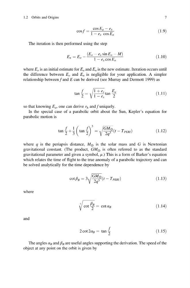
cos f ¼
cos E a À e x
1 À e x cos E a
ð1:9Þ
The iteration is then performed using the step
E n ¼ E o À
E o À e x sin E o À M
ð
Þ
1 À e x cos E o
ð1:10Þ
where E o is an initial estimate for E a and E n is the new estimate. Iteration occurs until
the difference between E o and E n is negligible for your application. A simpler
relationship between f and E can be derived (see Murray and Dermott 1999) as
tan
f
2
¼
ffiffiffiffiffiffiffiffiffiffiffiffi ffi
1 þ e x
1 À e x
r
tan
E a
2
ð1:11Þ
so that knowing E a , one can derive r h and f uniquely.
In the special case of a parabolic orbit about the Sun, Kepler’s equation for
parabolic motion is
tan
f
2
þ
1
3
tan
f
2
3
¼
ffiffiffiffiffiffiffiffiffiffiffi
GM ⨀
2q 3
r
t À T PERI
ð
Þ
ð 1:12Þ
where q is the periapsis distance, M ⨀ is the solar mass and G is Newtonian
gravitational constant. (The product, GM ⨀ is often referred to as the standard
gravitational parameter and given a symbol, μ.) This is a form of Barker’s equation
which relates the time of flight to the true anomaly of a parabolic trajectory and can
be solved analytically for the time dependence by
cot β B ¼ 3
ffiffiffiffiffiffiffiffiffiffiffi
GM ⨀
2q 3
r
t À T PERI
ð
Þ
ð 1:13Þ
where
ffiffiffiffiffiffiffiffiffiffiffiffiffi
cot
β B
2
3
r
¼ cot α B
ð1:14Þ
and
2 cot 2α B ¼ tan
f
2
ð1:15Þ
The angles α B and β B are useful angles supporting the derivation. The speed of the
object at any point on the orbit is given by
1.2 Orbits and Origins
7
cos E a À e x
1 À e x cos E a
ð1:9Þ
The iteration is then performed using the step
E n ¼ E o À
E o À e x sin E o À M
ð
Þ
1 À e x cos E o
ð1:10Þ
where E o is an initial estimate for E a and E n is the new estimate. Iteration occurs until
the difference between E o and E n is negligible for your application. A simpler
relationship between f and E can be derived (see Murray and Dermott 1999) as
tan
f
2
¼
ffiffiffiffiffiffiffiffiffiffiffiffi ffi
1 þ e x
1 À e x
r
tan
E a
2
ð1:11Þ
so that knowing E a , one can derive r h and f uniquely.
In the special case of a parabolic orbit about the Sun, Kepler’s equation for
parabolic motion is
tan
f
2
þ
1
3
tan
f
2
3
¼
ffiffiffiffiffiffiffiffiffiffiffi
GM ⨀
2q 3
r
t À T PERI
ð
Þ
ð 1:12Þ
where q is the periapsis distance, M ⨀ is the solar mass and G is Newtonian
gravitational constant. (The product, GM ⨀ is often referred to as the standard
gravitational parameter and given a symbol, μ.) This is a form of Barker’s equation
which relates the time of flight to the true anomaly of a parabolic trajectory and can
be solved analytically for the time dependence by
cot β B ¼ 3
ffiffiffiffiffiffiffiffiffiffiffi
GM ⨀
2q 3
r
t À T PERI
ð
Þ
ð 1:13Þ
where
ffiffiffiffiffiffiffiffiffiffiffiffiffi
cot
β B
2
3
r
¼ cot α B
ð1:14Þ
and
2 cot 2α B ¼ tan
f
2
ð1:15Þ
The angles α B and β B are useful angles supporting the derivation. The speed of the
object at any point on the orbit is given by
1.2 Orbits and Origins
7