

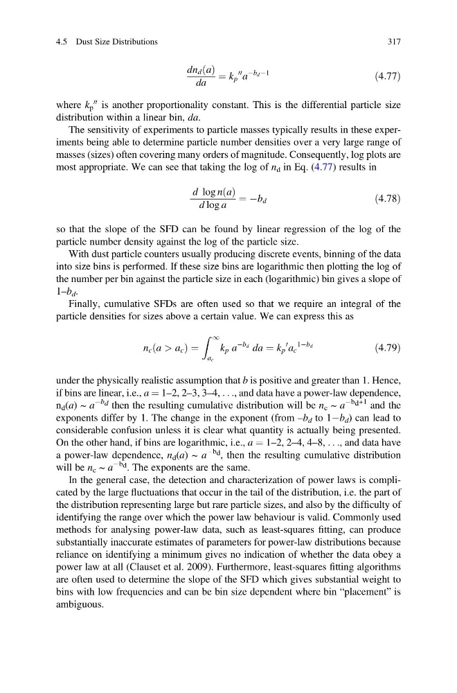
dn d a
ð Þ
da
¼ k p
00 a
Àb d À1
ð4:77Þ
where k p
00 is another proportionality constant. This is the differential particle size
distribution within a linear bin, da.
The sensitivity of experiments to particle masses typically results in these experiments being able to determine particle number densities over a very large range of
masses (sizes) often covering many orders of magnitude. Consequently, log plots are
most appropriate. We can see that taking the log of n d in Eq. (4.77) results in
d log n a
ð Þ
d log a
¼ Àb d
ð4:78Þ
so that the slope of the SFD can be found by linear regression of the log of the
particle number density against the log of the particle size.
With dust particle counters usually producing discrete events, binning of the data
into size bins is performed. If these size bins are logarithmic then plotting the log of
the number per bin against the particle size in each (logarithmic) bin gives a slope of
1–b d .
Finally, cumulative SFDs are often used so that we require an integral of the
particle densities for sizes above a certain value. We can express this as
n c a > a c
ð
Þ¼
Z 1
a c
k p a
Àb d da ¼ k p
0 a c
1Àb d
ð4:79Þ
under the physically realistic assumption that b is positive and greater than 1. Hence,
if bins are linear, i.e., a ¼ 1–2, 2–3, 3–4, . . ., and data have a power-law dependence,
n d (a) ~ a
Àb d then the resulting cumulative distribution will be n c ~ a
Àb d +1 and the
exponents differ by 1. The change in the exponent (from –b d to 1Àb d ) can lead to
considerable confusion unless it is clear what quantity is actually being presented.
On the other hand, if bins are logarithmic, i.e., a ¼ 1–2, 2–4, 4–8, . . ., and data have
a power-law dependence, n d (a) ~ a
Àb d , then the resulting cumulative distribution
will be n c ~ a
Àb d . The exponents are the same.
In the general case, the detection and characterization of power laws is complicated by the large fluctuations that occur in the tail of the distribution, i.e. the part of
the distribution representing large but rare particle sizes, and also by the difficulty of
identifying the range over which the power law behaviour is valid. Commonly used
methods for analysing power-law data, such as least-squares fitting, can produce
substantially inaccurate estimates of parameters for power-law distributions because
reliance on identifying a minimum gives no indication of whether the data obey a
power law at all (Clauset et al. 2009). Furthermore, least-squares fitting algorithms
are often used to determine the slope of the SFD which gives substantial weight to
bins with low frequencies and can be bin size dependent where bin “placement” is
ambiguous.
4.5 Dust Size Distributions
317
ð Þ
da
¼ k p
00 a
Àb d À1
ð4:77Þ
where k p
00 is another proportionality constant. This is the differential particle size
distribution within a linear bin, da.
The sensitivity of experiments to particle masses typically results in these experiments being able to determine particle number densities over a very large range of
masses (sizes) often covering many orders of magnitude. Consequently, log plots are
most appropriate. We can see that taking the log of n d in Eq. (4.77) results in
d log n a
ð Þ
d log a
¼ Àb d
ð4:78Þ
so that the slope of the SFD can be found by linear regression of the log of the
particle number density against the log of the particle size.
With dust particle counters usually producing discrete events, binning of the data
into size bins is performed. If these size bins are logarithmic then plotting the log of
the number per bin against the particle size in each (logarithmic) bin gives a slope of
1–b d .
Finally, cumulative SFDs are often used so that we require an integral of the
particle densities for sizes above a certain value. We can express this as
n c a > a c
ð
Þ¼
Z 1
a c
k p a
Àb d da ¼ k p
0 a c
1Àb d
ð4:79Þ
under the physically realistic assumption that b is positive and greater than 1. Hence,
if bins are linear, i.e., a ¼ 1–2, 2–3, 3–4, . . ., and data have a power-law dependence,
n d (a) ~ a
Àb d then the resulting cumulative distribution will be n c ~ a
Àb d +1 and the
exponents differ by 1. The change in the exponent (from –b d to 1Àb d ) can lead to
considerable confusion unless it is clear what quantity is actually being presented.
On the other hand, if bins are logarithmic, i.e., a ¼ 1–2, 2–4, 4–8, . . ., and data have
a power-law dependence, n d (a) ~ a
Àb d , then the resulting cumulative distribution
will be n c ~ a
Àb d . The exponents are the same.
In the general case, the detection and characterization of power laws is complicated by the large fluctuations that occur in the tail of the distribution, i.e. the part of
the distribution representing large but rare particle sizes, and also by the difficulty of
identifying the range over which the power law behaviour is valid. Commonly used
methods for analysing power-law data, such as least-squares fitting, can produce
substantially inaccurate estimates of parameters for power-law distributions because
reliance on identifying a minimum gives no indication of whether the data obey a
power law at all (Clauset et al. 2009). Furthermore, least-squares fitting algorithms
are often used to determine the slope of the SFD which gives substantial weight to
bins with low frequencies and can be bin size dependent where bin “placement” is
ambiguous.
4.5 Dust Size Distributions
317