

Ƥ ¼
ffiffiffiffiffiffiffiffiffiffiffiffiffiffiffiffiffiffiffiffiffiffiffiffiffiffiffiffi
Q
2
þ U
2
þ V
2
p
I
ð4:12Þ
and we can separate this into the degree of linear polarization
Ƥ L ¼
ffiffiffiffiffiffiffiffiffiffiffiffiffiffiffiffiffi
Q
2
þ U
2
p
I
ð4:13Þ
and the degree of circular polarization
Ƥ C ¼
V
I
ð4:14Þ
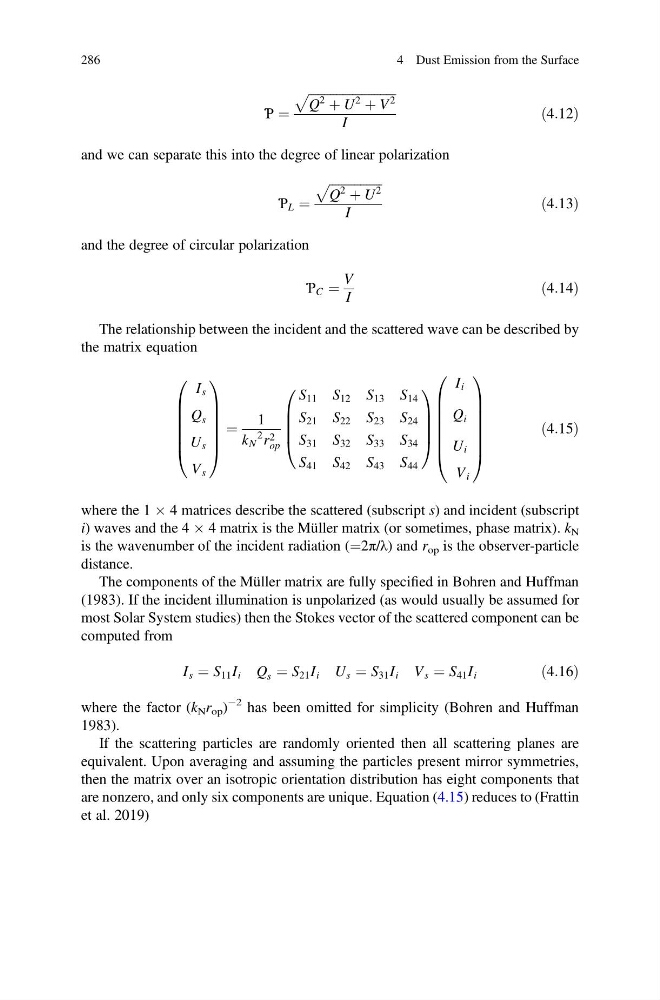
The relationship between the incident and the scattered wave can be described by
the matrix equation
I s
Q s
U s
V s
0
B
B
B
B
B
@
1
C
C
C
C
C
A
¼
1
k N
2 r 2
op
S 11 S 12 S 13 S 14
S 21 S 22 S 23 S 24
S 31 S 32 S 33 S 34
S 41 S 42 S 43 S 44
0
B
B
B
@
1
C
C
C
A
I i
Q i
U i
V i
0
B
B
B
B
B
B
@
1
C
C
C
C
C
C
A
ð4:15Þ
where the 1 Â 4 matrices describe the scattered (subscript s) and incident (subscript
i) waves and the 4 Â 4 matrix is the Müller matrix (or sometimes, phase matrix). k N
is the wavenumber of the incident radiation (¼2π/λ) and r op is the observer-particle
distance.
The components of the Müller matrix are fully specified in Bohren and Huffman
(1983). If the incident illumination is unpolarized (as would usually be assumed for
most Solar System studies) then the Stokes vector of the scattered component can be
computed from
I s ¼ S 11 I i Q s ¼ S 21 I i U s ¼ S 31 I i V s ¼ S 41 I i
ð4:16Þ
where the factor (k N r op )
À2 has been omitted for simplicity (Bohren and Huffman
1983).
If the scattering particles are randomly oriented then all scattering planes are
equivalent. Upon averaging and assuming the particles present mirror symmetries,
then the matrix over an isotropic orientation distribution has eight components that
are nonzero, and only six components are unique. Equation (4.15) reduces to (Frattin
et al. 2019)
286
4 Dust Emission from the Surface
ffiffiffiffiffiffiffiffiffiffiffiffiffiffiffiffiffiffiffiffiffiffiffiffiffiffiffiffi
Q
2
þ U
2
þ V
2
p
I
ð4:12Þ
and we can separate this into the degree of linear polarization
Ƥ L ¼
ffiffiffiffiffiffiffiffiffiffiffiffiffiffiffiffiffi
Q
2
þ U
2
p
I
ð4:13Þ
and the degree of circular polarization
Ƥ C ¼
V
I
ð4:14Þ
The relationship between the incident and the scattered wave can be described by
the matrix equation
I s
Q s
U s
V s
0
B
B
B
B
B
@
1
C
C
C
C
C
A
¼
1
k N
2 r 2
op
S 11 S 12 S 13 S 14
S 21 S 22 S 23 S 24
S 31 S 32 S 33 S 34
S 41 S 42 S 43 S 44
0
B
B
B
@
1
C
C
C
A
I i
Q i
U i
V i
0
B
B
B
B
B
B
@
1
C
C
C
C
C
C
A
ð4:15Þ
where the 1 Â 4 matrices describe the scattered (subscript s) and incident (subscript
i) waves and the 4 Â 4 matrix is the Müller matrix (or sometimes, phase matrix). k N
is the wavenumber of the incident radiation (¼2π/λ) and r op is the observer-particle
distance.
The components of the Müller matrix are fully specified in Bohren and Huffman
(1983). If the incident illumination is unpolarized (as would usually be assumed for
most Solar System studies) then the Stokes vector of the scattered component can be
computed from
I s ¼ S 11 I i Q s ¼ S 21 I i U s ¼ S 31 I i V s ¼ S 41 I i
ð4:16Þ
where the factor (k N r op )
À2 has been omitted for simplicity (Bohren and Huffman
1983).
If the scattering particles are randomly oriented then all scattering planes are
equivalent. Upon averaging and assuming the particles present mirror symmetries,
then the matrix over an isotropic orientation distribution has eight components that
are nonzero, and only six components are unique. Equation (4.15) reduces to (Frattin
et al. 2019)
286
4 Dust Emission from the Surface