

close to the nucleus surface (and hence the change in v gp ) is not also taken into
account.
q p (r) corresponds to an integral
q p r
ð Þ ¼
Z 2π
0
Z π
Àπ
n gp r
ð Þv gp r dθ r cos θ dφ
ð3:109Þ
(where θ, φ are angles around the source) so that by assuming force-free radial
outflow we have
q p r
ð Þ ¼ 4πr
2 v gp n gp r
ð Þ
ð3:110Þ
and
n gp r
ð Þ ¼
Q g
4πr 2 v gp
e
Àβ 1 r
ð3:111Þ
thereby giving the local parent density, n gp (cf. Eq. 3.1).
In the general case, the daughter product will also have a finite lifetime which can
be included using a second scalelength,
q d r
ð Þ ¼ Q gp
β 1
β 2 À β 1
e
Àβ 1 r
À e
Àβ 2 r
À
Á
ð3:112Þ
in units of [molecule s
À1 ] where β 2 is the reciprocal scalelength of the daughter
species. This is the Haser model equation (Cochran 1985).
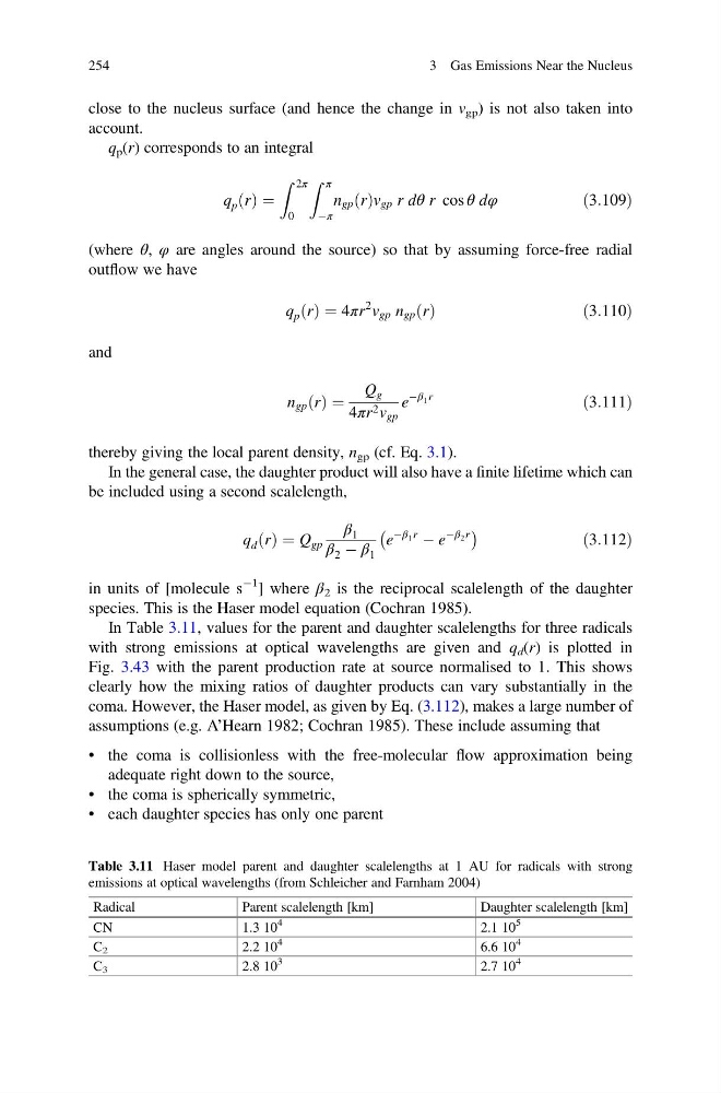
In Table 3.11, values for the parent and daughter scalelengths for three radicals
with strong emissions at optical wavelengths are given and q d (r) is plotted in
Fig. 3.43 with the parent production rate at source normalised to 1. This shows
clearly how the mixing ratios of daughter products can vary substantially in the
coma. However, the Haser model, as given by Eq. (3.112), makes a large number of
assumptions (e.g. A’Hearn 1982; Cochran 1985). These include assuming that
• the coma is collisionless with the free-molecular flow approximation being
adequate right down to the source,
• the coma is spherically symmetric,
• each daughter species has only one parent
Table 3.11 Haser model parent and daughter scalelengths at 1 AU for radicals with strong
emissions at optical wavelengths (from Schleicher and Farnham 2004)
Radical
Parent scalelength [km]
Daughter scalelength [km]
CN
1.3 10
4
2.1 10
5
C 2
2.2 10
4
6.6 10
4
C 3
2.8 10
3
2.7 10
4
254
3 Gas Emissions Near the Nucleus
account.
q p (r) corresponds to an integral
q p r
ð Þ ¼
Z 2π
0
Z π
Àπ
n gp r
ð Þv gp r dθ r cos θ dφ
ð3:109Þ
(where θ, φ are angles around the source) so that by assuming force-free radial
outflow we have
q p r
ð Þ ¼ 4πr
2 v gp n gp r
ð Þ
ð3:110Þ
and
n gp r
ð Þ ¼
Q g
4πr 2 v gp
e
Àβ 1 r
ð3:111Þ
thereby giving the local parent density, n gp (cf. Eq. 3.1).
In the general case, the daughter product will also have a finite lifetime which can
be included using a second scalelength,
q d r
ð Þ ¼ Q gp
β 1
β 2 À β 1
e
Àβ 1 r
À e
Àβ 2 r
À
Á
ð3:112Þ
in units of [molecule s
À1 ] where β 2 is the reciprocal scalelength of the daughter
species. This is the Haser model equation (Cochran 1985).
In Table 3.11, values for the parent and daughter scalelengths for three radicals
with strong emissions at optical wavelengths are given and q d (r) is plotted in
Fig. 3.43 with the parent production rate at source normalised to 1. This shows
clearly how the mixing ratios of daughter products can vary substantially in the
coma. However, the Haser model, as given by Eq. (3.112), makes a large number of
assumptions (e.g. A’Hearn 1982; Cochran 1985). These include assuming that
• the coma is collisionless with the free-molecular flow approximation being
adequate right down to the source,
• the coma is spherically symmetric,
• each daughter species has only one parent
Table 3.11 Haser model parent and daughter scalelengths at 1 AU for radicals with strong
emissions at optical wavelengths (from Schleicher and Farnham 2004)
Radical
Parent scalelength [km]
Daughter scalelength [km]
CN
1.3 10
4
2.1 10
5
C 2
2.2 10
4
6.6 10
4
C 3
2.8 10
3
2.7 10
4
254
3 Gas Emissions Near the Nucleus