

212
H. Wittig
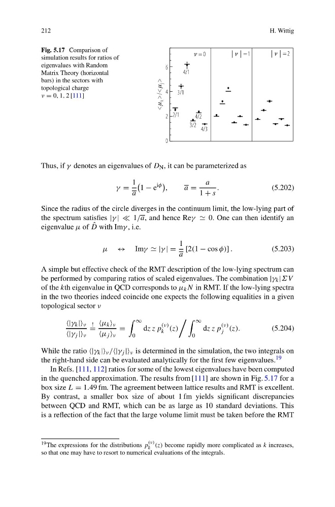
Fig. 5.17 Comparison of
simulation results for ratios of
eigenvalues with Random
Matrix Theory (horizontal
bars) in the sectors with
topological charge
ν = 0, 1, 2 [111]
4/2
4/3
3/2
2/1
3/1
4/1
6
4
2
0
> <
/
>
< j
k
= 0
=1
=2
Thus, if γ denotes an eigenvalues of D N , it can be parameterized as
γ =
1
a
1 − e
iφ
,
a =
a
1 + s
.
(5.202)
Since the radius of the circle diverges in the continuum limit, the low-lying part of
the spectrum satisfies |γ | | 1/a, and hence Reγ 0. One can then identify an
eigenvalue μ of ˆ
D with Imγ , i.e.
μ ↔ Imγ |γ | =
1
a
[2(1 − cos φ)] .
(5.203)
A simple but effective check of the RMT description of the low-lying spectrum can
be performed by comparing ratios of scaled eigenvalues. The combination |γ k |ΣV
of the kth eigenvalue in QCD corresponds to μ k N in RMT. If the low-lying spectra
in the two theories indeed coincide one expects the following equalities in a given
topological sector ν
k || ν
j || ν
!
=
k ν
j ν
≡
∞
0
dz z p
(ν)
k (z)
∞
0
dz z p
(ν)
j (z).
(5.204)
While the ratio k || ν / j || ν is determined in the simulation, the two integrals on
the right-hand side can be evaluated analytically for the first few eigenvalues. 19
In Refs. [111, 112] ratios for some of the lowest eigenvalues have been computed
in the quenched approximation. The results from [111] are shown in Fig. 5.17 for a
box size L = 1.49 fm. The agreement between lattice results and RMT is excellent.
By contrast, a smaller box size of about 1 fm yields significant discrepancies
between QCD and RMT, which can be as large as 10 standard deviations. This
is a reflection of the fact that the large volume limit must be taken before the RMT
19 The expressions for the distributions p
(ν)
k (z) become rapidly more complicated as k increases,
so that one may have to resort to numerical evaluations of the integrals.
H. Wittig
Fig. 5.17 Comparison of
simulation results for ratios of
eigenvalues with Random
Matrix Theory (horizontal
bars) in the sectors with
topological charge
ν = 0, 1, 2 [111]
4/2
4/3
3/2
2/1
3/1
4/1
6
4
2
0
> <
/
>
< j
k
= 0
=1
=2
Thus, if γ denotes an eigenvalues of D N , it can be parameterized as
γ =
1
a
1 − e
iφ
,
a =
a
1 + s
.
(5.202)
Since the radius of the circle diverges in the continuum limit, the low-lying part of
the spectrum satisfies |γ | | 1/a, and hence Reγ 0. One can then identify an
eigenvalue μ of ˆ
D with Imγ , i.e.
μ ↔ Imγ |γ | =
1
a
[2(1 − cos φ)] .
(5.203)
A simple but effective check of the RMT description of the low-lying spectrum can
be performed by comparing ratios of scaled eigenvalues. The combination |γ k |ΣV
of the kth eigenvalue in QCD corresponds to μ k N in RMT. If the low-lying spectra
in the two theories indeed coincide one expects the following equalities in a given
topological sector ν
k || ν
j || ν
!
=
k ν
j ν
≡
∞
0
dz z p
(ν)
k (z)
∞
0
dz z p
(ν)
j (z).
(5.204)
While the ratio k || ν / j || ν is determined in the simulation, the two integrals on
the right-hand side can be evaluated analytically for the first few eigenvalues. 19
In Refs. [111, 112] ratios for some of the lowest eigenvalues have been computed
in the quenched approximation. The results from [111] are shown in Fig. 5.17 for a
box size L = 1.49 fm. The agreement between lattice results and RMT is excellent.
By contrast, a smaller box size of about 1 fm yields significant discrepancies
between QCD and RMT, which can be as large as 10 standard deviations. This
is a reflection of the fact that the large volume limit must be taken before the RMT
19 The expressions for the distributions p
(ν)
k (z) become rapidly more complicated as k increases,
so that one may have to resort to numerical evaluations of the integrals.