

186
H. Wittig
Time
Time
Space
Space
L
0
C
C
( x x box with periodic b.c. )
L L L
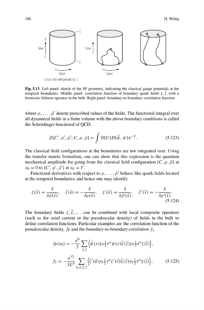
Fig. 5.13 Left panel: sketch of the SF geometry, indicating the classical gauge potentials at the
temporal boundaries. Middle panel: correlation function of boundary quark fields ζ, ¯
ζ with a
fermionic bilinear operator in the bulk. Right panel: boundary-to-boundary correlation function
where ρ, . . . , ¯
ρ denote prescribed values of the fields. The functional integral over
all dynamical fields in a finite volume with the above boundary conditions is called
the Schrödinger functional of QCD:
Z[C
, ρ
, ¯
ρ
; C, ρ, ¯
ρ] =
D[U ]D[ ¯
ψ, ψ] e
−S .
(5.123)
The classical field configurations at the boundaries are not integrated over. Using
the transfer matrix formalism, one can show that this expression is the quantum
mechanical amplitude for going from the classical field configuration {C, ρ, ¯
ρ} at
x 0 = 0 to {C , ρ , ¯
ρ } at x 0 = T .
Functional derivatives with respect to ρ, . . . , ¯
ρ behave like quark fields located
at the temporal boundaries, and hence one may identify
ζ( x) =
δ
δ ¯
ρ( x)
, ¯
ζ ( x) = −
δ
δρ( x)
, ζ
( x) =
δ
δ ¯
ρ ( x)
, ¯
ζ
( x) = −
δ
δρ ( x)
.
(5.124)
The boundary fields ζ, ¯
ζ , . . . can be combined with local composite operators
(such as the axial current or the pseudoscalar density) of fields in the bulk to
define correlation functions. Particular examples are the correlation function of the
pseudoscalar density, f P and the boundary-to-boundary correlation f 1
f P (x 0 ) = −
a 6
3
y, z
¯
ψ(x)γ 5
1
2 τ
a ψ(x) ¯
ζ ( y)γ 5
1
2 τ
a ζ( z)
,
f 1 = −
a 12
3L 6
u, v, y, z
¯
ζ
( u)γ 5
1
2 τ
a ζ
( v) ¯
ζ ( y)γ 5
1
2 τ
a ζ( z)
,
(5.125)
H. Wittig
Time
Time
Space
Space
L
0
C
C
( x x box with periodic b.c. )
L L L
Fig. 5.13 Left panel: sketch of the SF geometry, indicating the classical gauge potentials at the
temporal boundaries. Middle panel: correlation function of boundary quark fields ζ, ¯
ζ with a
fermionic bilinear operator in the bulk. Right panel: boundary-to-boundary correlation function
where ρ, . . . , ¯
ρ denote prescribed values of the fields. The functional integral over
all dynamical fields in a finite volume with the above boundary conditions is called
the Schrödinger functional of QCD:
Z[C
, ρ
, ¯
ρ
; C, ρ, ¯
ρ] =
D[U ]D[ ¯
ψ, ψ] e
−S .
(5.123)
The classical field configurations at the boundaries are not integrated over. Using
the transfer matrix formalism, one can show that this expression is the quantum
mechanical amplitude for going from the classical field configuration {C, ρ, ¯
ρ} at
x 0 = 0 to {C , ρ , ¯
ρ } at x 0 = T .
Functional derivatives with respect to ρ, . . . , ¯
ρ behave like quark fields located
at the temporal boundaries, and hence one may identify
ζ( x) =
δ
δ ¯
ρ( x)
, ¯
ζ ( x) = −
δ
δρ( x)
, ζ
( x) =
δ
δ ¯
ρ ( x)
, ¯
ζ
( x) = −
δ
δρ ( x)
.
(5.124)
The boundary fields ζ, ¯
ζ , . . . can be combined with local composite operators
(such as the axial current or the pseudoscalar density) of fields in the bulk to
define correlation functions. Particular examples are the correlation function of the
pseudoscalar density, f P and the boundary-to-boundary correlation f 1
f P (x 0 ) = −
a 6
3
y, z
¯
ψ(x)γ 5
1
2 τ
a ψ(x) ¯
ζ ( y)γ 5
1
2 τ
a ζ( z)
,
f 1 = −
a 12
3L 6
u, v, y, z
¯
ζ
( u)γ 5
1
2 τ
a ζ
( v) ¯
ζ ( y)γ 5
1
2 τ
a ζ( z)
,
(5.125)