

174
H. Wittig
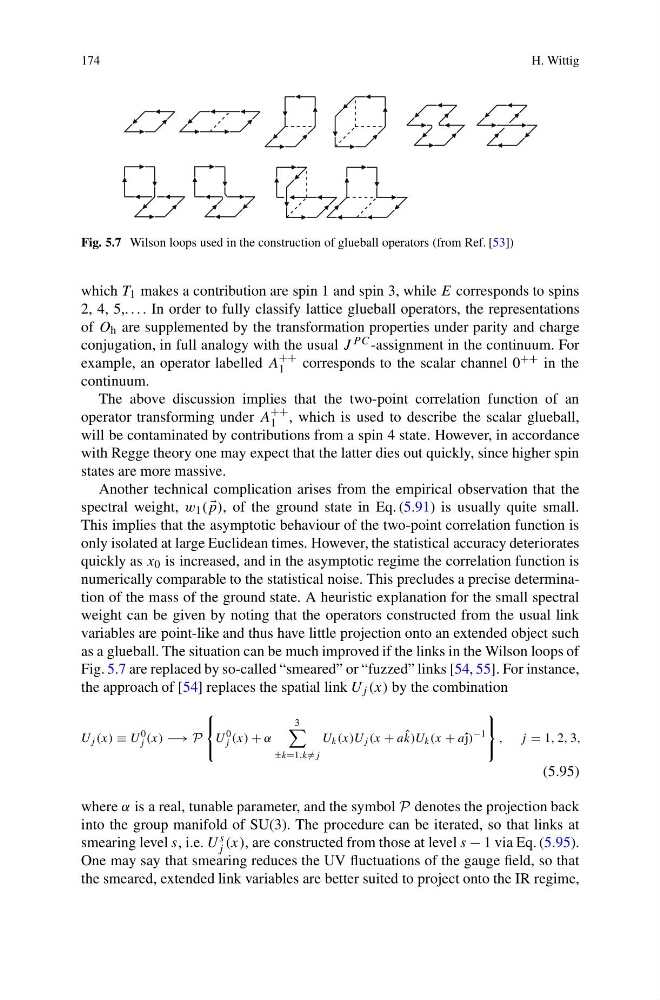
Fig. 5.7 Wilson loops used in the construction of glueball operators (from Ref. [53])
which T 1 makes a contribution are spin 1 and spin 3, while E corresponds to spins
2, 4, 5,. . . . In order to fully classify lattice glueball operators, the representations
of O h are supplemented by the transformation properties under parity and charge
conjugation, in full analogy with the usual J P C -assignment in the continuum. For
example, an operator labelled A
++
1
corresponds to the scalar channel 0 ++ in the
continuum.
The above discussion implies that the two-point correlation function of an
operator transforming under A
++
1 , which is used to describe the scalar glueball,
will be contaminated by contributions from a spin 4 state. However, in accordance
with Regge theory one may expect that the latter dies out quickly, since higher spin
states are more massive.
Another technical complication arises from the empirical observation that the
spectral weight, w 1 (
p), of the ground state in Eq. (5.91) is usually quite small.
This implies that the asymptotic behaviour of the two-point correlation function is
only isolated at large Euclidean times. However, the statistical accuracy deteriorates
quickly as x 0 is increased, and in the asymptotic regime the correlation function is
numerically comparable to the statistical noise. This precludes a precise determination of the mass of the ground state. A heuristic explanation for the small spectral
weight can be given by noting that the operators constructed from the usual link
variables are point-like and thus have little projection onto an extended object such
as a glueball. The situation can be much improved if the links in the Wilson loops of
Fig. 5.7 are replaced by so-called “smeared” or “fuzzed” links [54, 55]. For instance,
the approach of [54] replaces the spatial link U j (x) by the combination
U j (x) ≡ U
0
j (x) −→ P
⎧
⎨
⎩
U
0
j (x) + α
3
±k=1,k =j
U k (x)U j (x + a ˆ
k)U k (x + aˆ j)
−1
⎫
⎬
⎭
, j = 1, 2, 3,
(5.95)
where α is a real, tunable parameter, and the symbol P denotes the projection back
into the group manifold of SU(3). The procedure can be iterated, so that links at
smearing level s, i.e. U
s
j (x), are constructed from those at level s − 1 via Eq. (5.95).
One may say that smearing reduces the UV fluctuations of the gauge field, so that
the smeared, extended link variables are better suited to project onto the IR regime,
H. Wittig
Fig. 5.7 Wilson loops used in the construction of glueball operators (from Ref. [53])
which T 1 makes a contribution are spin 1 and spin 3, while E corresponds to spins
2, 4, 5,. . . . In order to fully classify lattice glueball operators, the representations
of O h are supplemented by the transformation properties under parity and charge
conjugation, in full analogy with the usual J P C -assignment in the continuum. For
example, an operator labelled A
++
1
corresponds to the scalar channel 0 ++ in the
continuum.
The above discussion implies that the two-point correlation function of an
operator transforming under A
++
1 , which is used to describe the scalar glueball,
will be contaminated by contributions from a spin 4 state. However, in accordance
with Regge theory one may expect that the latter dies out quickly, since higher spin
states are more massive.
Another technical complication arises from the empirical observation that the
spectral weight, w 1 (
p), of the ground state in Eq. (5.91) is usually quite small.
This implies that the asymptotic behaviour of the two-point correlation function is
only isolated at large Euclidean times. However, the statistical accuracy deteriorates
quickly as x 0 is increased, and in the asymptotic regime the correlation function is
numerically comparable to the statistical noise. This precludes a precise determination of the mass of the ground state. A heuristic explanation for the small spectral
weight can be given by noting that the operators constructed from the usual link
variables are point-like and thus have little projection onto an extended object such
as a glueball. The situation can be much improved if the links in the Wilson loops of
Fig. 5.7 are replaced by so-called “smeared” or “fuzzed” links [54, 55]. For instance,
the approach of [54] replaces the spatial link U j (x) by the combination
U j (x) ≡ U
0
j (x) −→ P
⎧
⎨
⎩
U
0
j (x) + α
3
±k=1,k =j
U k (x)U j (x + a ˆ
k)U k (x + aˆ j)
−1
⎫
⎬
⎭
, j = 1, 2, 3,
(5.95)
where α is a real, tunable parameter, and the symbol P denotes the projection back
into the group manifold of SU(3). The procedure can be iterated, so that links at
smearing level s, i.e. U
s
j (x), are constructed from those at level s − 1 via Eq. (5.95).
One may say that smearing reduces the UV fluctuations of the gauge field, so that
the smeared, extended link variables are better suited to project onto the IR regime,