

154
H. Wittig
to the continuum limit, the algorithmic efficiency, the renormalization properties of
local operators, or—in the case of domain wall fermions—the extent to which chiral
symmetry is realized. Depending on the properties of a particular discretization, the
choice of lattice action can be optimized for the physics one wishes to study.
5.2.3 Functional Integral and Observables
The lattice formulation provides a regularization of non-Abelian gauge theories
whilst preserving the gauge invariance at all stages of the calculation. This comes
at a price, since all continuous space-time symmetries are broken explicitly and
must be recovered in the continuum limit. Nevertheless, the lattice regularized
theory inherits all consequences of gauge invariance, including renormalizability.
Moreover, the lattice regularizes the theory without any reference to perturbation
theory. By contrast, in continuum schemes like the MS scheme of dimensional
regularization the cutoff is only defined after fixing the order of the perturbative
expansion. As we shall see below, observables in lattice QCD are directly given
in terms of functional integrals, which can be evaluated stochastically using Monte
Carlo integration. In this way, any use of perturbation theory is completely avoided.
For concreteness, let us assume that we have made a particular choice for
the Yang–Mills part S G [U ] and the fermionic part S F [U, ¯
ψ, ψ], for instance, the
Wilson plaquette action and Wilson fermions. Let denote an observable, which is
represented by a polynomial in the quark and antiquark fields and the link variables.
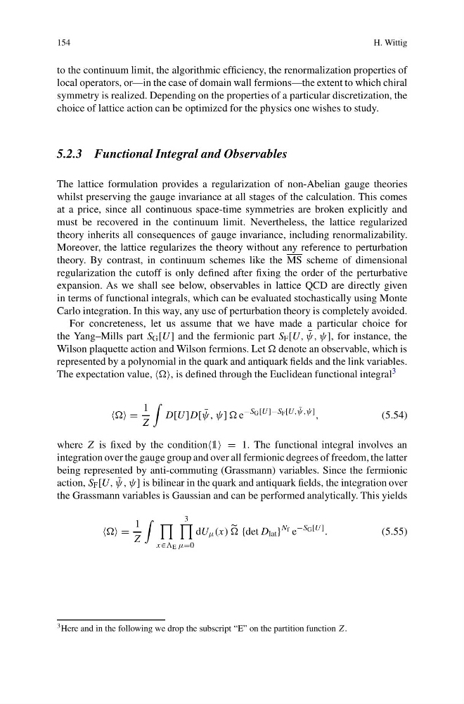
The expectation value, is defined through the Euclidean functional integral 3
=
1
Z
D[U ]D[ ¯
ψ, ψ] e
−S G [U ]−S F [U, ¯
ψ,ψ] ,
(5.54)
where Z is fixed by the condition = 1. The functional integral involves an
integration over the gauge group and over all fermionic degrees of freedom, the latter
being represented by anti-commuting (Grassmann) variables. Since the fermionic
action, S F [U, ¯
ψ, ψ] is bilinear in the quark and antiquark fields, the integration over
the Grassmann variables is Gaussian and can be performed analytically. This yields
=
1
Z
x∈ E
3
μ=0
dU μ (x)
{det D lat }
N f e
−S G [U ] .
(5.55)
3 Here and in the following we drop the subscript “E” on the partition function Z.
H. Wittig
to the continuum limit, the algorithmic efficiency, the renormalization properties of
local operators, or—in the case of domain wall fermions—the extent to which chiral
symmetry is realized. Depending on the properties of a particular discretization, the
choice of lattice action can be optimized for the physics one wishes to study.
5.2.3 Functional Integral and Observables
The lattice formulation provides a regularization of non-Abelian gauge theories
whilst preserving the gauge invariance at all stages of the calculation. This comes
at a price, since all continuous space-time symmetries are broken explicitly and
must be recovered in the continuum limit. Nevertheless, the lattice regularized
theory inherits all consequences of gauge invariance, including renormalizability.
Moreover, the lattice regularizes the theory without any reference to perturbation
theory. By contrast, in continuum schemes like the MS scheme of dimensional
regularization the cutoff is only defined after fixing the order of the perturbative
expansion. As we shall see below, observables in lattice QCD are directly given
in terms of functional integrals, which can be evaluated stochastically using Monte
Carlo integration. In this way, any use of perturbation theory is completely avoided.
For concreteness, let us assume that we have made a particular choice for
the Yang–Mills part S G [U ] and the fermionic part S F [U, ¯
ψ, ψ], for instance, the
Wilson plaquette action and Wilson fermions. Let denote an observable, which is
represented by a polynomial in the quark and antiquark fields and the link variables.
The expectation value, is defined through the Euclidean functional integral 3
=
1
Z
D[U ]D[ ¯
ψ, ψ] e
−S G [U ]−S F [U, ¯
ψ,ψ] ,
(5.54)
where Z is fixed by the condition = 1. The functional integral involves an
integration over the gauge group and over all fermionic degrees of freedom, the latter
being represented by anti-commuting (Grassmann) variables. Since the fermionic
action, S F [U, ¯
ψ, ψ] is bilinear in the quark and antiquark fields, the integration over
the Grassmann variables is Gaussian and can be performed analytically. This yields
=
1
Z
x∈ E
3
μ=0
dU μ (x)
{det D lat }
N f e
−S G [U ] .
(5.55)
3 Here and in the following we drop the subscript “E” on the partition function Z.