

4 QCD: The Theory of Strong Interactions
101
logarithmically at large Q 2 (asymptotic freedom), while in QED the coupling has
the opposite behaviour.
4.4 More on the Running Coupling
In the previous section we have introduced the renormalised coupling α in terms of
the 3-gluon vertex at p 2 = −μ 2 (momentum subtraction). The Ward identities of
QCD then ensure that the coupling defined from other vertices like the ¯
qqg vertex
are renormalised in the same way and the finite radiative corrections are related.
But at present the universally adopted definition of α s is in terms of dimensional
regularisation because of computational simplicity which is essential given the great
complexity of present day calculations. So we now briefly review the principles
of dimensional regularisation and the definition of Minimal Subtraction (MS) and
Modified Minimal Subtraction (MS). The MS definition of α s is the one most
commonly adopted in the literature and a value quoted for it is nomally referring
to this definition.
Dimensional Regularisation (DR) is a gauge and Lorentz invariant regularisation
that consists in formulating the theory in D < 4 spacetime dimensions in order to
make loop integrals ultraviolet finite. In DR one rewrites the theory in D dimensions
(D is integer at the beginning, but then we will see that the expression of diagrams
makes sense at all D except for isolated singularities). The metric tensor is extended
into a D × D matrix g μν = diag(1, −1, −1, . . . ., −1) and 4-vectors are given by
k μ = (k 0 , k 1 , . . . , k D−1 ). The Dirac γ μ are f (D) × f (D) matrices and it is not
important what is the precise form of the function f (D). It is sufficient to extend
the usual algebra in a straightforward way like {γ μ , γ ν } = 2g μ,ν I , with I the Ddimensional identity matrix, γ μ γ ν γ μ = −(D − 2)γ ν or T r(γ μ γ ν ) = f (D)g μν .
The physical dimensions of fields change in D dimensions and, as a consequence,
the gauge couplings become dimensional e D = μ e, where e is dimensionless,
D = 4 − 2 and μ is a scale of mass (this is how a scale of mass is introduced in
the DR of massless QCD!). The dimension of fields is determined by requiring that
the action S =
d D xL is dimensionless. By inserting for L terms like m ¯
or
m 2 φ † φ or e ¯
μ μ the dimensions of the fields and coupling are determined as:
m, ,, φ, A μ , e = 1, (D − 1)/2, (D − 2)/2, (D − 2)/2, (4 − D)/2, respectively.
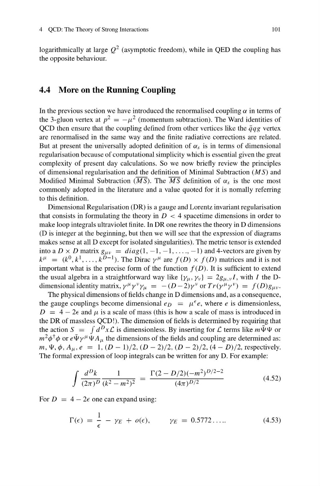
The formal expression of loop integrals can be written for any D. For example:
d D k
(2π) D
1
(k 2 − m 2 ) 2 =
− D/2)(−m 2 ) D/2−2
(4π) D/2
(4.52)
For D = 4 − 2 one can expand using:
=
1
− γ E + o((),
γ E = 0.5772 . . . ..
(4.53)
101
logarithmically at large Q 2 (asymptotic freedom), while in QED the coupling has
the opposite behaviour.
4.4 More on the Running Coupling
In the previous section we have introduced the renormalised coupling α in terms of
the 3-gluon vertex at p 2 = −μ 2 (momentum subtraction). The Ward identities of
QCD then ensure that the coupling defined from other vertices like the ¯
qqg vertex
are renormalised in the same way and the finite radiative corrections are related.
But at present the universally adopted definition of α s is in terms of dimensional
regularisation because of computational simplicity which is essential given the great
complexity of present day calculations. So we now briefly review the principles
of dimensional regularisation and the definition of Minimal Subtraction (MS) and
Modified Minimal Subtraction (MS). The MS definition of α s is the one most
commonly adopted in the literature and a value quoted for it is nomally referring
to this definition.
Dimensional Regularisation (DR) is a gauge and Lorentz invariant regularisation
that consists in formulating the theory in D < 4 spacetime dimensions in order to
make loop integrals ultraviolet finite. In DR one rewrites the theory in D dimensions
(D is integer at the beginning, but then we will see that the expression of diagrams
makes sense at all D except for isolated singularities). The metric tensor is extended
into a D × D matrix g μν = diag(1, −1, −1, . . . ., −1) and 4-vectors are given by
k μ = (k 0 , k 1 , . . . , k D−1 ). The Dirac γ μ are f (D) × f (D) matrices and it is not
important what is the precise form of the function f (D). It is sufficient to extend
the usual algebra in a straightforward way like {γ μ , γ ν } = 2g μ,ν I , with I the Ddimensional identity matrix, γ μ γ ν γ μ = −(D − 2)γ ν or T r(γ μ γ ν ) = f (D)g μν .
The physical dimensions of fields change in D dimensions and, as a consequence,
the gauge couplings become dimensional e D = μ e, where e is dimensionless,
D = 4 − 2 and μ is a scale of mass (this is how a scale of mass is introduced in
the DR of massless QCD!). The dimension of fields is determined by requiring that
the action S =
d D xL is dimensionless. By inserting for L terms like m ¯
or
m 2 φ † φ or e ¯
μ μ the dimensions of the fields and coupling are determined as:
m, ,, φ, A μ , e = 1, (D − 1)/2, (D − 2)/2, (D − 2)/2, (4 − D)/2, respectively.
The formal expression of loop integrals can be written for any D. For example:
d D k
(2π) D
1
(k 2 − m 2 ) 2 =
− D/2)(−m 2 ) D/2−2
(4π) D/2
(4.52)
For D = 4 − 2 one can expand using:
=
1
− γ E + o((),
γ E = 0.5772 . . . ..
(4.53)