

98
G. Altarelli and S. Forte
Z
−1
V Z
3/2
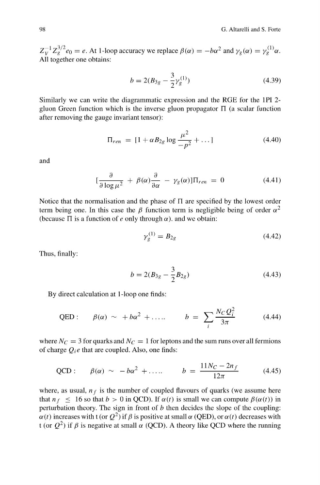
g e 0 = e. At 1-loop accuracy we replace β(α) = −bα 2 and γ g (α) = γ
(1)
g α.
All together one obtains:
b = 2(B 3g −
3
2
γ
(1)
g )
(4.39)
Similarly we can write the diagrammatic expression and the RGE for the 1PI 2gluon Green function which is the inverse gluon propagator (a scalar function
after removing the gauge invariant tensor):
ren = [1 + αB 2g log
μ 2
−p 2 + . . . ]
(4.40)
and
[
∂
∂ log μ 2 + β(α)
∂
∂α
− γ g (α)] ren = 0
(4.41)
Notice that the normalisation and the phase of are specified by the lowest order
term being one. In this case the β function term is negligible being of order α 2
(because is a function of e only through α). and we obtain:
γ
(1)
g = B 2g
(4.42)
Thus, finally:
b = 2(B 3g −
3
2
B 2g )
(4.43)
By direct calculation at 1-loop one finds:
QED :
β(α) ∼ + bα
2
+ . . . ..
b =
i
N C Q 2
i
3π
(4.44)
where N C = 3 for quarks and N C = 1 for leptons and the sum runs over all fermions
of charge Q i e that are coupled. Also, one finds:
QCD :
β(α) ∼ − bα
2
+ . . . ..
b =
11N C − 2n f
12π
(4.45)
where, as usual, n f is the number of coupled flavours of quarks (we assume here
that n f ≤ 16 so that b > 0 in QCD). If α(t) is small we can compute β(α(t)) in
perturbation theory. The sign in front of b then decides the slope of the coupling:
α(t) increases with t (or Q 2 ) if β is positive at small α (QED), or α(t) decreases with
t (or Q 2 ) if β is negative at small α (QCD). A theory like QCD where the running
G. Altarelli and S. Forte
Z
−1
V Z
3/2
g e 0 = e. At 1-loop accuracy we replace β(α) = −bα 2 and γ g (α) = γ
(1)
g α.
All together one obtains:
b = 2(B 3g −
3
2
γ
(1)
g )
(4.39)
Similarly we can write the diagrammatic expression and the RGE for the 1PI 2gluon Green function which is the inverse gluon propagator (a scalar function
after removing the gauge invariant tensor):
ren = [1 + αB 2g log
μ 2
−p 2 + . . . ]
(4.40)
and
[
∂
∂ log μ 2 + β(α)
∂
∂α
− γ g (α)] ren = 0
(4.41)
Notice that the normalisation and the phase of are specified by the lowest order
term being one. In this case the β function term is negligible being of order α 2
(because is a function of e only through α). and we obtain:
γ
(1)
g = B 2g
(4.42)
Thus, finally:
b = 2(B 3g −
3
2
B 2g )
(4.43)
By direct calculation at 1-loop one finds:
QED :
β(α) ∼ + bα
2
+ . . . ..
b =
i
N C Q 2
i
3π
(4.44)
where N C = 3 for quarks and N C = 1 for leptons and the sum runs over all fermions
of charge Q i e that are coupled. Also, one finds:
QCD :
β(α) ∼ − bα
2
+ . . . ..
b =
11N C − 2n f
12π
(4.45)
where, as usual, n f is the number of coupled flavours of quarks (we assume here
that n f ≤ 16 so that b > 0 in QCD). If α(t) is small we can compute β(α(t)) in
perturbation theory. The sign in front of b then decides the slope of the coupling:
α(t) increases with t (or Q 2 ) if β is positive at small α (QED), or α(t) decreases with
t (or Q 2 ) if β is negative at small α (QCD). A theory like QCD where the running