

668
L. Lyons
Table 15.1 Bayesian 90% confidence level upper limits for the production rate s as a function
of n, the observed number of events
n
b = 0.0
b = 3.0
0
2.35 (2.30)
2.35 (2.30)
3
6.87 (6.68)
4.46 (4.36)
6
10.88 (10.53)
7.80 (7.60)
9
14.71 (14.21)
11.56 (11.21)
20
28.27 (27.05)
25.05 (24.05)
The Poisson parameter μ = ∗ s + b, where the expected background b is either 0.0 or 3.0,
and is precisely known; and , whose true values is 1.0, is estimated in a subsidiary measurement
with 10% accuracy. The numbers in brackets are the corresponding upper limits when is known
precisely. At large n, the limits for b = 3.0 are 3 units lower than those for b = 0.0; the latter are
approximately n + 1.28
√
n at large n. The effect of the uncertainty in is to increase the limits,
and by a larger amount at large n. For n = 0, these Bayesian limits are independent of the expected
background b
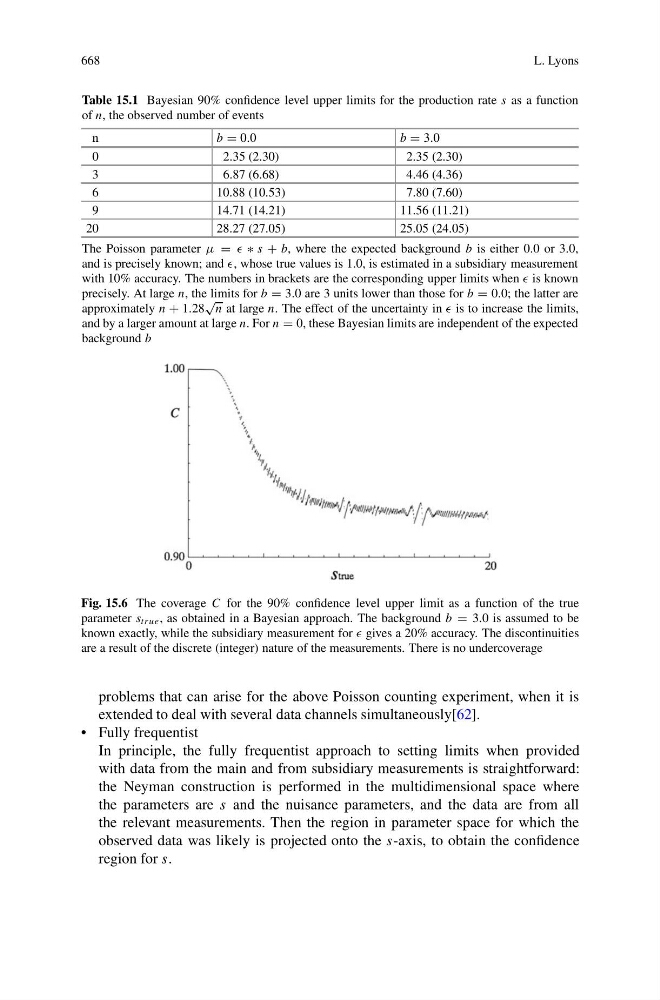
Fig. 15.6 The coverage C for the 90% confidence level upper limit as a function of the true
parameter s true , as obtained in a Bayesian approach. The background b = 3.0 is assumed to be
known exactly, while the subsidiary measurement for gives a 20% accuracy. The discontinuities
are a result of the discrete (integer) nature of the measurements. There is no undercoverage
problems that can arise for the above Poisson counting experiment, when it is
extended to deal with several data channels simultaneously[62].
• Fully frequentist
In principle, the fully frequentist approach to setting limits when provided
with data from the main and from subsidiary measurements is straightforward:
the Neyman construction is performed in the multidimensional space where
the parameters are s and the nuisance parameters, and the data are from all
the relevant measurements. Then the region in parameter space for which the
observed data was likely is projected onto the s-axis, to obtain the confidence
region for s.