

666
L. Lyons
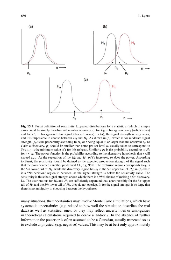
Fig. 15.5 Punzi definition of sensitivity. Expected distributions for a statistic t (which in simple
cases could be simply the observed number of events n), for H 0 = background only (solid curves)
and for H 1 = background plus signal (dashed curves). In (a), the signal strength is very weak,
and it is impossible to choose between H 0 and H 1 . As shown in (b), which is for moderate signal
strength, p 0 is the probability according to H 0 of t being equal to or larger than the observed t 0 . To
claim a discovery, p 0 should be smaller than some pre-set level α, usually taken to correspond to
5σ ; t crit is the minimum value of t for this to be so. Similarly p 1 is the probability according to H 1
for t ≤ t 0 . The power function is the probability according to the alternative hypothesis that t will
exceed t crit . As the separation of the H 0 and H 1 pdf s increases, so does the power. According
to Punzi, the sensitivity should be defined as the expected production strength of the signal such
that the power exceeds another predefined CL, e.g. 95%. The exclusion region corresponds to t 0 in
the 5% lower tail of H 1 , while the discovery region has t 0 in the 5σ upper tail of H 0 ; in (b) there
is a “No decision” region in between, as the signal strength is below the sensitivity value. The
sensitivity is thus the signal strength above which there is a 95% chance of making a 5σ discovery.
i.e. The distributions for H 0 and H 1 are sufficiently separated that, apart possibly for the 5σ upper
tail of H 0 and the 5% lower tail of H 1 , they do not overlap. In (c) the signal strength is so large that
there is no ambiguity in choosing between the hypotheses
many situations, the uncertainties may involve Monte Carlo simulations, which have
systematic uncertainties (e.g. related to how well the simulation describes the real
data) as well as statistical ones; or they may reflect uncertainties or ambiguities
in theoretical calculations required to derive b and/or . In the absence of further
information the posterior is often assumed to be a Gaussian, usually truncated so as
to exclude unphysical (e.g. negative) values. This may be at best only approximately