

13 Pattern Recognition and Reconstruction
557
−20
−10
0
10
20
−20
−10
0
10
20
x
y
−1
−0.5
0
0.5
1
−1
−0.5
0
0.5
1
u
v
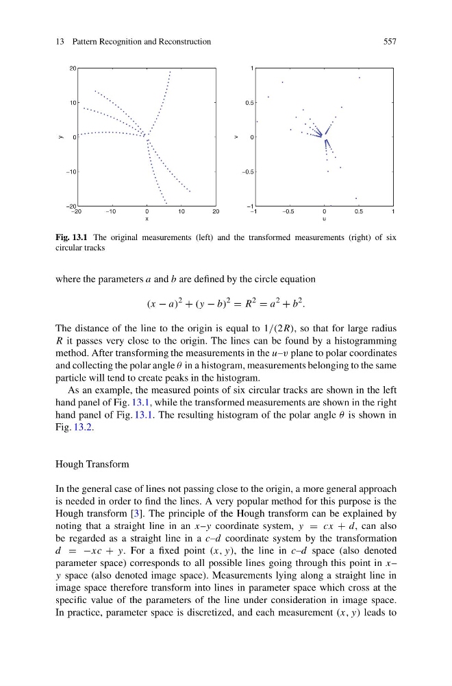
Fig. 13.1 The original measurements (left) and the transformed measurements (right) of six
circular tracks
where the parameters a and b are defined by the circle equation
(x − a)
2
+ (y − b)
2
= R
2
= a
2
+ b
2 .
The distance of the line to the origin is equal to 1/(2R), so that for large radius
R it passes very close to the origin. The lines can be found by a histogramming
method. After transforming the measurements in the u–v plane to polar coordinates
and collecting the polar angle θ in a histogram, measurements belonging to the same
particle will tend to create peaks in the histogram.
As an example, the measured points of six circular tracks are shown in the left
hand panel of Fig. 13.1, while the transformed measurements are shown in the right
hand panel of Fig. 13.1. The resulting histogram of the polar angle θ is shown in
Fig. 13.2.
Hough Transform
In the general case of lines not passing close to the origin, a more general approach
is needed in order to find the lines. A very popular method for this purpose is the
Hough transform [3]. The principle of the Hough transform can be explained by
noting that a straight line in an x–y coordinate system, y = cx + d, can also
be regarded as a straight line in a c–d coordinate system by the transformation
d = −xc + y. For a fixed point (x, y), the line in c–d space (also denoted
parameter space) corresponds to all possible lines going through this point in x–
y space (also denoted image space). Measurements lying along a straight line in
image space therefore transform into lines in parameter space which cross at the
specific value of the parameters of the line under consideration in image space.
In practice, parameter space is discretized, and each measurement (x, y) leads to
557
−20
−10
0
10
20
−20
−10
0
10
20
x
y
−1
−0.5
0
0.5
1
−1
−0.5
0
0.5
1
u
v
Fig. 13.1 The original measurements (left) and the transformed measurements (right) of six
circular tracks
where the parameters a and b are defined by the circle equation
(x − a)
2
+ (y − b)
2
= R
2
= a
2
+ b
2 .
The distance of the line to the origin is equal to 1/(2R), so that for large radius
R it passes very close to the origin. The lines can be found by a histogramming
method. After transforming the measurements in the u–v plane to polar coordinates
and collecting the polar angle θ in a histogram, measurements belonging to the same
particle will tend to create peaks in the histogram.
As an example, the measured points of six circular tracks are shown in the left
hand panel of Fig. 13.1, while the transformed measurements are shown in the right
hand panel of Fig. 13.1. The resulting histogram of the polar angle θ is shown in
Fig. 13.2.
Hough Transform
In the general case of lines not passing close to the origin, a more general approach
is needed in order to find the lines. A very popular method for this purpose is the
Hough transform [3]. The principle of the Hough transform can be explained by
noting that a straight line in an x–y coordinate system, y = cx + d, can also
be regarded as a straight line in a c–d coordinate system by the transformation
d = −xc + y. For a fixed point (x, y), the line in c–d space (also denoted
parameter space) corresponds to all possible lines going through this point in x–
y space (also denoted image space). Measurements lying along a straight line in
image space therefore transform into lines in parameter space which cross at the
specific value of the parameters of the line under consideration in image space.
In practice, parameter space is discretized, and each measurement (x, y) leads to